Shape-based Segmentation of Tomatoes for Agriculture Monitoring

Ujjwal Verma

1,2

, Florence Rossant

, Isabelle Bloch

, Julien Orensanz

and Denis Boisgontier

ISEP, Paris, France

Institut Mines-Telecom, T

ecom ParisTech, CNRS LTCI, Paris, France

Cap2020, Gironville sur Essonne, France

Keywords:

Image Segmentation, Parametric Active Contours, Shape Constraint, Precision Farming, Elliptic Approxima-

tion.

Abstract:

In this paper, we present a segmentation procedure based on a parametric active contour with shape constraint,

in order to follow the growth of the tomatoes from the images acquired in the ﬁeld. This is a challenging task

because of the poor contrast in the images and the occlusions by the vegetation. In our sequential approach,

considering one image per day, we assume that a segmentation of the tomatoes is available for the image

acquired the previous day. An initial curve for the active contour model is computed by combining gradient

information and region information. Then, an active contour with shape constraint is applied to provide an

elliptic approximation of the tomato boundary. We performed a quantitative evaluation of our approach by

comparing the results with the manual segmentation. Given the varying degree of occlusion in the images, the

image data set was divided into three categories, based on the occlusion degree of the tomato in the processed

image. For the cases with low occlusion, good results were obtained, with an average relative distance between

the manual segmentation and the automatic segmentation of 2.73% (expressed as percentage of the size of

tomato). For the images with signiﬁcant amount of occlusion, a good segmentation was obtained on 44% of

the images, where the average error was less than 10%.

1 INTRODUCTION

Optimal harvesting date and predicted yield are valu-

able information when farming open ﬁeld tomatoes,

making harvest planning and work at the process-

ing plant much easier. Monitoring tomatoes during

their early stages of growth is also interesting to as-

sess plant stress or abnormal development. Satellite

data and crop growth modeling are generally used for

estimating the yield of a large region (Prasad et al.,

2006),(Mkhabela et al., 2011). However, satellite data

are affected by adverse climatic conditions (clouds,

etc.) resulting in inaccurate predictions(Mkhabela

et al., 2011). Crop growth modeling, which inte-

grates information regarding the cultivated plant, soil

and weather conditions, considers the ideal case with

no infected plant. Recent studies have concentrated

on combining these two approaches(Zhao and Pei,

2013). Nevertheless these methods depend on the

quality of the different parameters involved (vegeta-

tion indices, soil and weather information) and they

are not accurate enough to detect abnormal develop-

ment.

In this work, we present a different approach

where we intend to monitor the growth of tomatoes

and measure their size in an open ﬁeld. For this pur-

pose, two cameras are installed in the ﬁeld and two

images are captured at regular intervals. In order to

avoid a complete 3D reconstruction, we assume that a

tomato can be approximated by a sphere in the 3D

space, which projects into an ellipse in the image

plane. Hence, the ﬁrst part of our system aims at de-

tecting and segmenting the tomatoes in both images,

using elliptic approximations. Then, the second part

aims at estimating the sphere radius, using the camera

parameters. An estimate of the yield is obtained from

this information. In this paper, we focus on the seg-

mentation procedure only.

Computer vision algorithms have been applied in

the agricultural domain in order to replace human op-

erators with an automated system. They have been

used to grade and sort agricultural products (Jayas

et al., 2000; Du and Sun, 2006; Narendra and Ha-

reesh, 2010), to detect weeds in a ﬁeld (Aitkenhead

et al., 2003; Yang et al., 2000; Lee et al., 1999), and

to model the growth of fruits and then predict the

402

Verma U., Rossant F., Bloch I., Orensanz J. and Boisgontier D..

Shape-based Segmentation of Tomatoes for Agriculture Monitoring.

DOI: 10.5220/0004818804020411

In Proceedings of the 3rd International Conference on Pattern Recognition Applications and Methods (ICPRAM-2014), pages 402-411

ISBN: 978-989-758-018-5

 2014 SCITEPRESS (Science and Technology Publications, Lda.)

yield (Aggelopoulou et al., 2011; Stajnko and Cme-

lik, 2005). In (Aggelopoulou et al., 2011), the yield

of an apple orchard is estimated using only the den-

sity of ﬂowers. In (Stajnko and Cmelik, 2005), only 5

images captured at different stages of the apple matu-

ration are studied in order to predict the yield. How-

ever, to the best of our knowledge, there has not been

any related work where the growth of a fruit or veg-

etable is studied based on the images captured during

the entire agricultural season.

There is little growth of a tomato during a given

day. So, only one image per day is analyzed in this

work, thus creating a series of images (approximately

20-30 images). One of the difﬁculties of the segmen-

tation part is occlusion: most of the tomatoes are par-

tially hidden by other tomatoes and/or leaves (Figure

1). Moreover, color information is not of much use as

tomatoes are red only at the end of the ripening. Also,

another difﬁculty is a very low contrast in some cases

due to shadows.

(a) 6

image. (b) 7

image.

Figure 1: Two successive images of the tomato S = 7.

In this work, the segmentation should be as auto-

matic as possible. However, we assume that an opera-

tor validates each obtained segmentation. If the result

is poor, the operator rejects it. Indeed, given the dif-

ﬁculties, the segmentation is a very challenging task,

and a manual validation is preferable. This approach

enables us to use the segmentation done in the i

im-

age (if validated) as a reference for the segmentation

of the same tomato in the (i + 1)

image.

In order to segment the tomatoes, we use a para-

metric active contour model, which allows us to in-

troduce a priori knowledge on the shape of the object

to be segmented, thus making the segmentation more

robust to noise and occlusion. Using an elliptic shape

constraint is consistent with our prior assumption.

The main steps of the segmentation algorithm are

the following: ﬁrst, gradient information is used in or-

der to ﬁnd the candidate contour points and propose

several elliptic approximations using the RANSAC

algorithm. Secondly, region information is added, en-

abling us to select the best ellipse for the initialization

of the active contour and ﬁnding the regions of poten-

tial occlusions. Third, the active contour with elliptic

constraint is applied. Finally, four ellipse estimates

are computed. The operator has only to select the best

one as the ﬁnal segmentation.

The original features of the proposed algorithm in-

clude the approximation of the tomatoes as ellipses

and the conditioning of the computation of the image

energy by the non-occluded regions. These features

allow coping with occlusions and local loss of con-

tour and edges.

We present the active contour model with shape

constraint in Section 2 and the different steps of the

segmentation algorithm in Section 3. Section 4 dis-

cusses the experimental results.

2 ACTIVE CONTOUR WITH AN

ELLIPTICAL SHAPE PRIOR

Parametric active contour model or snake was orig-

inally introduced by (Kass et al., 1988) in order to

detect a boundary of an object in an image. This al-

gorithm deforms the contour iteratively from its initial

position towards the edges of an object by minimiz-

ing an energy functional. The energy functional asso-

ciated with the contour v is usually composed of three

terms:

(v) = E

(v) + E

Ext

(v) (1)

where E

(v) is the internal energy controlling the

smoothness of the curve and E

(v) is the energy de-

rived from image data. The external energy E

Ext

(v)

can express contextual information, such as shape in-

formation. The authors in (Foulonneau et al., 2006)

used Legendre moments to deﬁne an afﬁne invariant

shape prior in a region based active contour. In our

case, the region information is not signiﬁcant due to

the presence of leaves (occlusions) and other toma-

toes of similar intensity proﬁle. In (Charmi et al.,

2009), Fourier descriptors are used in order to align

the active contour with the reference curve of suit-

able shape and orientation. In our work, the tomato

in each image is assumed to have an ellipse shape.

Since ellipses are easily represented in a parametric

form from a few parameters, it is natural to propose a

parametric active contour model.

Let us deﬁne the reference ellipse as z

. This el-

lipse is estimated from the evolving contour z. Both

curves are expressed in polar coordinates with the ori-

gin at the center of z

(θ) = r

(θ)e

jθ

, z(θ) = r(θ)e

jθ

, θ ∈ [0, 2π] (2)

Shape-basedSegmentationofTomatoesforAgricultureMonitoring

403

Our energy functional with an elliptic shape regular-

ization is deﬁned as:

(r, r

) =

2π

(θ)|

dθ +

2π

(r(θ)e

jθ

)dθ

2π

|r(θ) − r

(θ)|

dθ (3)

In the above equation, the ﬁrst term represents the in-

ternal energy which controls the variations of r and

makes it regular. The second term is a classical image

energy calculated from the gradient vector ﬂow (Xu

and Prince, 1998). The last term restricts the evolving

contour to be close to the reference ellipse. The pa-

rameter α controls the smoothness of the curve, and

ψ controls the inﬂuence of the shape prior on the total

energy. Note that instead of modifying a 2-D vector

v(s) = (x(s), y(s)) as in the classical active contour

model, only a 1-D vector r(θ) is modiﬁed for each

value of the parameter θ. Moreover, the shape con-

straint makes the usual second derivative term in the

internal energy useless, and is therefore not included

in the proposed energy functional.

The minimum of E

is obtained in two steps:

First, a least square estimate of the ellipse z

is com-

puted from the initial contour z

. Then, the evolving

contour z is computed by minimizing E

while as-

suming z

ﬁxed. From the evolving contour z so ob-

tained, the parameters of the least square estimate of

the ellipse z

are regularly updated. This two-step it-

erative process is repeated, in order to obtain the min-

imum of E

The minimization of E

with respect to r is equiv-

alent to solving the following Euler equation:

−αr

(θ)+∇E

(θ)·n(θ)+ψ(r(θ)−r

(θ)) = 0 (4)

where n(θ) = [cosθ, sin θ]

To ﬁnd iteratively a solution of this equation, we

introduce a time variable, and the resulting equation

is discretized using ﬁnite differences, as in the case of

the classical active contours.

3 DETAILED ALGORITHM

In this section, we present an algorithm which allows

us to follow the growth of a tomato, which has been

manually segmented in the ﬁrst image (i = 1).

Let us denote by im

i+1

the (i + 1)

image of the

tomato S. In the rest of this paper, an ellipse cen-

tered at [xc,yc], whose semi major and minor axes

lengths are a and b, respectively, and which has a rota-

tion angle of ϕ, is represented as Ell = [xc, yc, a, b, ϕ].

The tomato approximated by an ellipse in im

is rep-

resented as Ell

= [xc

, yc

, a

, b

, ϕ

]. In our sequen-

tial approach, the computation of the contour in the

(i + 1)

image is based on both the information in

i+1

and the contour of the tomato in the i

image.

In the following sections, it is assumed that there is

little movement and little growth of tomatoes between

two successive images (Figure 2).

3.1 Pre-processing

As mentioned above, the color information is not of

much use. However, the edges of tomatoes are more

prominent in the red component of the image, and

hence only this component is considered. The orig-

inal image is cropped around the position (xc

, yc

resulting in a smaller image (imS

i+1

). The contrast is

enhanced by a contrast stretching transformation.

3.2 Updating the Tomato Position

Due to its increasing weight, the tomato tends to

fall towards the ground (Figure 2) and its position

in imS

i+1

is calculated, using pattern matching. The

bright areas, that may correspond to the tomato, are

extracted by convolving the cropped image with a

binary mask representing a white disk of radius χr

where

+ b

(5)

and χ is a constant determined experimentally. The

local maxima C

i+1

= {(x

, y

), k = 1, ..., k

} are then

extracted. From these k

points, the one C

, y

), which is the closest to (xc

, yc

), is selected

as the new location of the tomato center (Figure 2(b)).

A new cropped image imS

i+1

is then extracted

from im

i+1

, centered at C

= (x

, y

). The size of

this new image is adapted to the size of the tomato

(deduced from a

and b

) so that we restrict the region

to be analyzed as much as possible, reducing thus the

processing cost of the next steps. The contrast stretch-

ing transformation is applied to imS

i+1

(a) 7

image. (b) 8

image.

Figure 2: Updating the position of the tomato: previous po-

sition (xc

, yc

) in red, candidate positions C

i+1

in magenta

and blue, and new position C

in blue.

ICPRAM2014-InternationalConferenceonPatternRecognitionApplicationsandMethods

404

3.3 Elliptic Approximations

In order to obtain an initial contour for the active con-

tour model, we ﬁrst compute l

points which may lie

on the boundary of the tomato. From these l

points,

a RANSAC estimate is used to obtain several candi-

date ellipses. Finally, one of these ellipses is selected

as the initial contour based on additional region infor-

mation and size regularization (Section 3.4.2).

3.3.1 Detection of Tomato Contour Points

Let us take C

as the origin of the polar coordinate

system. Then we select l

points P

= p

jθ

, where

l = 1, ..., l

, 0 < θ

< 2π, that satisfy the following

three conditions:

0.5r

< p

< 1.5r

(6)

|arg(∇imS

i+1

)) − θ

| ≤

(7)

|∇imS

i+1

)| > η (8)

where ∇imS

i+1

) is the gradient at P

in imS

i+1

. The

above conditions select the points of strong gradient

whose direction is within an acceptable limit with re-

spect to the vector normal to the circle with radius

. The threshold values have been set experimen-

tally. As shown in Figure 5(a), most points lying on

the boundary of the tomato have been correctly de-

tected along with some additional points lying on the

leaves.

3.3.2 Calculation of Several Ellipses from the

Points P

using RANSAC Estimation

A least square estimate of an ellipse calculated from

all l

points might result in a contour far away from

the actual boundary because of the detection of irrel-

evant points. Therefore, we use a RANSAC (Fischler

and Bolles, 1981) estimate based on an elliptic model

in order to compute several candidate ellipses.

Under normal circumstances, the size and the ori-

entation of the tomato in imS

i+1

are supposed to be

close to the ones in imS

. This information is incorpo-

rated in the RANSAC estimation and only the ellipses

whose parameters satisfy the following conditions are

considered:

−0.1 <

i+1

− a

< 0.2, −0.1 <

i+1

− b

< 0.2 (9)

−0.1 <

i+1

− SA

< 0.25 (10)

Ecc

i+1

− Ecc

Ecc

| < 0.1 (11)

i+1

− ϕ

| < 0.2 (12)

where SA

i+1

and SA

represent the surface of the el-

lipses in imS

i+1

and imS

respectively. The eccentric-

ity (Ecc =

) for the two ellipses is denoted by Ecc

i+1

and Ecc

respectively.

Negative variations for a and b (Equation 9) are

possible because of the movement of the tomato with

respect to the camera or because of the variation in the

orientation, as tomatoes are actually not perfect spher-

ical objects. Equation 10 restricts the apparent size of

the tomato while Equation 11 restricts the admissible

values for eccentricity, thus controlling the apparent

shape of the tomato.

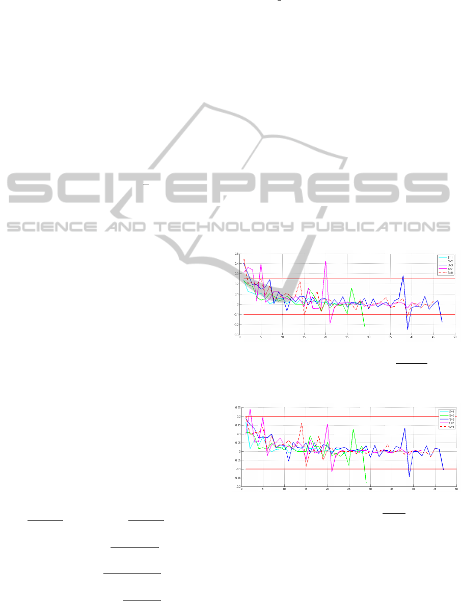
The threshold values in Equations 9-12 have been

determined after studying the parameters of the el-

lipses obtained from the manual segmentation of ﬁve

tomatoes. For example, Figures 3 and 4 shows

the relative evolution of the surface SA and length

of semi-major axis a of the ellipses. Most of the

measurements are situated within the limits deﬁned

above. Note that the dissymmetry in the lower and

upper bounds in Equations 9-10 is due to the fact that

tomatoes are supposed to grow during the agricultural

season.

Figure 3: Evolution of SA. The abscissa represents the im-

age number (i), and the ordinate represents

i+1

−SA

. The

solid horizontal red lines show the selected threshold val-

ues.

Figure 4: Evolution of a. The abscissa represents the image

number (i), and the ordinate represents

i+1

−a

. The solid

horizontal red lines show the selected threshold values.

From the N ellipses computed using the RANSAC

algorithm, a total of N

ellipses, with N

< N, are

retained, corresponding to the N

ellipses with the

largest number of inliers (Figure 5(b)).

Shape-basedSegmentationofTomatoesforAgricultureMonitoring

405

(a) P

points detected. (b) N

= 20) ellipses.

Figure 5: Points of strong gradient and ellipses detected us-

ing the RANSAC estimate.

3.4 Adding Region Information

A region growing algorithm is applied in order to

add region information and determine the best initial-

ization for the active contour among the N

ellipses

Ell

i+1

, where u = 1, ..., N

. Moreover, potential oc-

clusions are also derived from this information.

3.4.1 Using Region Growing to Calculate the

Region Representing a Tomato

Let us denote by ω

the binary image representing the

region inside the ellipse Ell

i+1

. We apply a classical

region growing algorithm starting from ω

seed

and lim-

iting the growing to ω

limit

, where:

seed

u=1

, ω

limit

[

u=1

(13)

The ﬁnal region is denoted by ω

(Figure 6(a)).

3.4.2 Selecting the Initial Contour

We deﬁne τ

as:

= min

u=1,2,....N

τ(u) (14)

with

τ(u) =

|ω

∩ (1 − ω

)| + |(1 − ω

) ∩ ω

|ω

∩ ω

(15)

where |A| represents the cardinality of a set A. τ(u)

measures the consistency between the segmentation

obtained through the contour analysis ω

and the re-

gion analysis ω

. It reaches a minimum (zero) when

and ω

match perfectly.

Let us denote by a

i+1

and b

i+1

the axes lengths

of the candidate ellipse Ell

i+1

, u ∈ [1, N

]. We

select the ellipse v (Figure 6(b)) that minimizes



i+1

− a

)

+ (b

i+1

− b



under the condition

τ(v) ≤ 1.1 τ

(16)

Thus, we have obtained the initial contour by com-

bining the results obtained using two different seg-

mentation methods, one based on boundary informa-

tion and the other based on region information. The

selected ellipse Ell

i+1

is chosen among the ones for

which both results are consistent, allowing therefore

a better robustness with respect to occlusions. More-

over, another regularization condition is added, which

imposes that the size and shape of the ellipse in imS

i+1

are close to the ones in imS

(a) ω

. (b) Ell

i+1

Figure 6: Result of the region growing (ω

) and selection of

the initial ellipse Ell

i+1

3.4.3 Finding Potential Occlusion

This part aims at ﬁnding the regions where occlusions

could disturb the behavior of the active contour. For

example, the region in which the tomato is attached to

the plant has a different intensity from the one of the

tomato.

Let Ell

denote the ellipse which covers the con-

vex hull of ω

and which minimizes the number of

pixels inside the ellipse Ell

and not belonging to the

region ω

(Figure 7(a)). Let ω

be the region inside

Ell

. Then, the region of occlusion ω

can be com-

puted as:

= ω

∩ ω

(17)

Using morphological operations (erosion fol-

lowed by reconstruction by dilation), small regions

are removed from ω

, so that the resulting ω

corre-

sponds to actual leaves causing the occlusions (Figure

7(b)). Apart from detecting the “head” of the tomato,

any other additional occlusion (mostly due to leaves)

can also be detected using this approach (Figure 7(b)).

3.5 Applying Active Contours

The active contour (Section 2) is applied

with the following initialization Ell

i+1

[xc

i+1

, yc

i+1

, 0.95a

i+1

, 0.95b

i+1

, ϕ

i+1

]. Indeed,

the movement of the curve z is smoother and faster

if initialized inside the tomato. For the ﬁrst n

start

ICPRAM2014-InternationalConferenceonPatternRecognitionApplicationsandMethods

406

(a) Ell

. (b) ω

Figure 7: Detecting the regions of potential occlusion.

iterations, the parameter ψ is set to zero, so that z

moves towards the most prominent contours. Then

the shape constraint is introduced for n

ellipse

iterations

(ψ 6= 0) in order to guarantee robustness with respect

to occlusion. Finally, the shape constraint is relaxed

(ψ = 0) for a few n

end

iterations, which guarantees

reaching the boundary more accurately, as a tomato

is not a perfect ellipse.

Note that the image forces are not considered in

the region of occlusion ω

, in every step of this pro-

cess.

Updating the Reference Ellipse: As explained in

Section 2, the reference ellipse z

is updated every

shape

iterations. A least square estimate calculated

from all the points of the curve z is not relevant, be-

cause some of them may lie on false contours (e.g.

leaves). So, the following algorithm aims at selecting

a subset of points that actually lie on the boundary of

the tomato.

We use a polar coordinate system with the origin

at the center of the current reference ellipse z

. As in

Section 2, let us denote by z(θ) = r(θ)e

jθ

a point of

the evolving curve, z

(θ) = r

(θ)e

jθ

the correspond-

ing point on the reference ellipse, n

(θ) the vector

normal to the ellipse z

, and z

(θ) = r

(θ)e

jθ

the point

that maximizes the gradient module for 0 < r

(θ) <

1.1r

(θ). The point z(θ) is selected as a point lying on

the boundary of the tomato if it satisﬁes the following

conditions:

|∇imS

i+1

(z(θ)) · n

(θ)| > Γ (18)

|∇imS

i+1

(z(θ)) · n

(θ)|

|∇imS

i+1

(z(θ))|

> 0.75 (19)

d(z

(θ), z(θ)) < d

max

(20)

where · represents the vector dot product.

The ﬁrst condition ensures that the magnitude of

the gradient vector projected onto the normal of the

ellipse is strong. The threshold Γ is determined auto-

matically (Otsu, 1975). The second condition ensures

that the direction of the gradient is close to the vector

normal to the ellipse. The last condition (d

max

= 2 in

our experiments) imposes that the point considered is

a meaningful local maximum of the gradient. Finally,

the parameters of the reference ellipse are updated by

calculating a least square approximation from the sub-

set of points lying on the evolving contour z selected

using the above conditions (Figure 8(a)).

(a) Updating z

from se-

lected points (green).

(b) Final contour z.

Figure 8: Active contour with shape constraint.

3.6 Reﬁning the Results

A least square estimate of an ellipse from z (Fig-

ure 8(b)) is generally not relevant as outliers may be

present due to occlusion. So, again, a selection proce-

dure is applied. A ﬁrst subset of points P

is obtained

by using criteria similar to the ones described in Sec-

tion 3.5 (Equations 18-20) . Then, another subset P

is computed by relaxing the condition related to the

gradient direction (Figure 9).

(a) set of points P

. (b) Points P

Figure 9: Two different set of points P

and P

Final Contour: Then four ellipses are computed as

follows:

1. A least square approximation Ell

i+1

f 1

[xc

i+1

f 1

, yc

i+1

f 1

, a

i+1

f 1

, b

i+1

f 1

, ϕ

i+1

f 1

] is computed from

all the points of z.

2. Another estimate Ell

i+1

f 2

[xc

i+1

f 2

, yc

i+1

f 2

, a

i+1

f 2

, b

i+1

f 2

, ϕ

i+1

f 2

] is obtained from P

Shape-basedSegmentationofTomatoesforAgricultureMonitoring

407

using the RANSAC algorithm with the following

conditions:

0.9a

i+1

f 1

< a

i+1

f 2

< 1.1a

i+1

f 1

(21)

0.9b

i+1

f 1

< b

i+1

f 2

< 1.1b

i+1

f 1

(22)

3. A least square approximation Ell

i+1

f 3

is obtained

from the subset P

4. A weighted least square estimate Ell

i+1

f 4

is ob-

tained where the points of P

are assigned a higher

weight (0.75) and the other points of z a lower

weight (0.25). This is done in order to give impor-

tance to the points that are surely on the boundary

of the tomato.

If the images have a good contrast, and little or no oc-

clusion, all the four ellipses will be almost identical

(Figure 10(a)). However, in case of occlusions and

poor contrast, the four ellipses may be different (Fig-

ure 10(b)).

(a) 8

image. (b) 17

image: P

(yellow)

and P

(green).

Figure 10: Final ellipse estimates for two different images.

4 RESULTS

Two cameras (Pentax Optio W80) were installed in

an open ﬁeld of tomatoes. The same setup was used

for two agricultural seasons (April-August, 2011 and

2012), capturing one image per day. We have identi-

ﬁed 10 tomatoes, covering different sites and differ-

ent seasons, thus ensuring variability (302 images in

total). The tomatoes were identiﬁed manually by ob-

serving the images of the entire agricultural season.

Due to the severe occlusions, only a limited number of

tomatoes were visible in most of the images of a given

season. Therefore, only the tomatoes which were vis-

ible in more than 10 consecutive images were studied.

The obtained segmentations A were compared

with the manual segmentations M (approximated by

ellipses) by computing the average D

mean

and maxi-

mal D

max

distance between A and M for the i

im-

age (expressed in pixels). In order to better interpret

the results, the maximum and mean distances between

two contours are normalized by the size of the tomato

as:

meanR

mean

100 (23)

maxR

max

100 (24)

where r

is deﬁned in Equation 5.

The data set contains images of varying contrast

and degree of occlusions. Obviously, it is impossible

to obtain a reliable segmentation in case of severe oc-

clusion, even manually. Consequently we studied ex-

perimentally the effect of the percentage of occlusion

on the ﬁnal estimation of the radius of a spherical ob-

ject (considering the complete system, segmentation

and partial 3D reconstruction). In our experiments,

the percentage P of occlusion corresponds to the oc-

clusion of an arc with subtended angle equal to

2πP

100

For less than 30% occlusion, the variation in the esti-

mated radius was very small, and for more than 30%

occlusion, signiﬁcant change in the values of the esti-

mated radius was observed. Thus, we identiﬁed three

different categories:

• Category 1, containing images with an amount of

occlusion P less than 30% for which the estima-

tion is very robust with respect to segmentation

imprecision (Figure 11(a)),

• Category 2, with 30% < P < 50% which is more

prone to segmentation error (Figure 11(b)),

• Category 3, with P > 50% for which it is impos-

sible to perform a reliable segmentation (Figure

11(c)).

The percentage of occlusion was determined manu-

ally by selecting the end points of the occluded elliptic

arc. Note that the percentage of occlusion was com-

puted only to evaluate the segmentation procedure,

and this is not a part of the algorithm.

Table 1 shows the mean (µ) and the standard

deviation (σ) for D

meanR

and D

maxR

, for the images

belonging to category 1. Good results were ob-

tained even in the presence of occlusion by nearby

leaves/branches and tomatoes (Figures 12(a) and

12(b)). Also, a low µ

meanR

along with lower σ

meanR

demonstrates the robustness of the proposed method.

However, in some images captured at the beginning

of the season, when the size is very small, the

occlusion due to leaves present on the “head” of the

tomato results in an ambiguity on the position of the

actual contour (Figure 12(c)). Also, in some images

(Figure 12(d)), due to a shadow effect on a portion

of the contour, the intensity proﬁle of the tomato

and the adjacent leaves are nearly identical, resulting

in a very low contrast. Such cases may result in

ICPRAM2014-InternationalConferenceonPatternRecognitionApplicationsandMethods

408

(a) Category 1: Tomato S = 1,

Image 8.

(b) Category 2: Tomato S = 7,

Image 17.

Image 14.

Figure 11: Three different categories of image based on the

occlusion.

comparatively high distance measures even in the

absence of any occlusion.

In the images of category 2, containing a sig-

niﬁcant amount of occlusion, good results were

obtained on 44 % of the images (Figure 13), where

meanR

< 10%. For this category µ

meanR

lies in the

interval [2, 30]% for ellipse Ell

f 4

. The signiﬁcantly

higher distance measure for some images of this

category is caused by the false detection of the

position of the tomato due to the occlusion. The

position of the tomatoes was not correctly detected

in approximately 6% of the images belonging to

category 2. Note that Ell

f 4

is not necessarily the best

ellipse, and is selected for illustrative purpose only.

Due to the variation in the contrast and occlusion,

in general, there is not a single ellipse (among the

four ellipse estimates) which represents a good

segmentation for all the images. Let us denote by

Ell

opt

the ellipse, among the four ellipse estimates

(Ell

f 1

, Ell

f 2

, Ell

f 3

and Ell

f 4

), for which µ

meanR

minimum. Table 2 shows the distribution of D

meanR

and D

maxR

for ellipse Ell

opt

. It can be observed that

the values of D

meanR

and D

maxR

for Ell

opt

are lower

than for those of Ell

f 4

. This shows that there is at

least one ellipse among the four ellipse estimates

which best represents the tomato. The operator has

only to select the best ellipse.

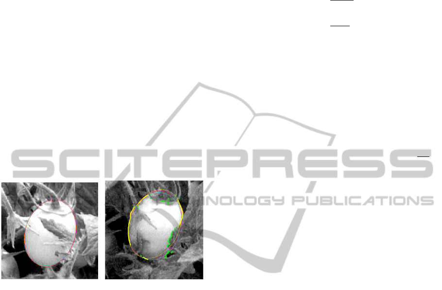
(a) Tomato S = 1, Image 8

(1.89%, 4.70%).

(b) Tomato S = 4, Image 24

(1.29%,4.39%).

(4.71%, 11.84%).

(d) Tomato S = 8, Image 5

(4.77%, 16.04%).

Figure 12: Final segmentation Ell

f 4

(red) obtained on im-

ages of category 1. The contour in cyan represents the man-

ual segmentation. Also shown are the distance measures.

The values in brackets are (D

meanR

, D

maxR

(a) Tomato S = 7, Image 17

(1.94%, 5.45%).

(b) Tomato S = 4, Image 18

(2.22%,6.16%).

Figure 13: Final segmentation Ell

f 4

(red) obtained on im-

ages of category 2.

5 CONCLUSIONS

We presented a segmentation procedure used to

monitor tomatoes in images. Starting from an

approximate computation of the position of the center

of the tomato, segmentation algorithms based on

contour and region information are proposed and

combined, in order to determine a ﬁrst estimate of the

contour. Then, a parametric active contour with shape

constraint is applied and four ellipse estimates repre-

senting the tomatoes are obtained. In all the steps of

this process, a priori knowledge about the shape and

Shape-basedSegmentationofTomatoesforAgricultureMonitoring

409

the size of the tomatoes is modeled and incorporated

as regularization terms, leading to better robustness.

It is supposed that the operator selects, at the end of

the process for each image, the ellipse correspond-

ing to the best elliptic estimation of the actual contour.

Table 1: Mean (µ) and standard deviation (σ) of D

meanR

and

maxR

by comparing ellipse Ell

f 4

with the manual segmen-

tation M. Only the images belonging to category 1 (i.e. with

a low amount of occlusion) have been considered.

meanR

maxR

S = 1 26 1.72 0.77 5.06 2.76

S = 2 4 1.85 0.46 5.45 1.91

S = 3 21 3.40 2.24 9.79 6.88

S = 4 14 2.73 1.92 7.81 5.71

S = 5 5 4.81 1.30 13.05 3.56

S = 6 0 - - - -

S = 7 25 1.88 0.65 4.81 1.97

S = 8 20 6.07 5.75 15.41 10.61

S = 9 1 5.26 0.00 11.86 0.00

S = 10 5 2.25 0.56 6.59 2.25

Table 2: Mean (µ) and standard deviation (σ) of D

meanR

and

maxR

by comparing ellipse Ell

opt

with the manual segmen-

tation M. Only the images belonging to category 1 (i.e. with

a low amount of occlusion) have been considered.

meanR

maxR

S = 1 26 1.34 0.68 3.76 2.21

S = 2 4 1.57 0.4 4.43 0.88

S = 3 21 2.87 2.05 8.4 6.58

S = 4 14 2.2 1.77 6.28 5.34

S = 5 5 4.54 1.14 12.44 3.46

S = 6 0 - - - -

S = 7 25 1.7 0.49 4.61 1.62

S = 8 20 5.4 4.88 14.9 10.37

S = 9 1 5.24 0 11.86 0

S = 10 5 1.75 0.36 4.4 1.25

The segmentation of tomatoes is a challenging

task due to the presence of occlusion and variation

in contrast. In order to evaluate the robustness of the

proposed algorithm, the entire image set was divided

into three categories based on the amount of occlu-

sion. For the images with an acceptable level of occlu-

sion, good results were obtained with an average vari-

ation in D

meanR

less than 6%. Also, the low standard

deviation for D

meanR

indicates the robustness of the

proposed algorithm. Good results with D

meanR

< 10%

were obtained on 44% of the images which contain a

signiﬁcant amount of occlusion.

For the moment, it has been assumed that an oper-

ator manually selects one ellipse as the ﬁnal segmen-

tation. In future work, we wish to provide automati-

cally the best representation of the tomato. Also, in

some images, the position of the tomato is not de-

tected correctly due to the presence of other toma-

toes nearby. This could be improved by updating the

position of the tomato globally by considering also

the movement of adjacent tomatoes. One possible

improvement for the active contour model is to re-

strict the size of the reference ellipse, as there is little

growth between two consecutive images.

ACKNOWLEDGEMENTS

This work is partially supported by European Re-

gional Development Fund (ERDF).

REFERENCES

Aggelopoulou, A., Bochtis, D., Fountas, S., Swain, K.,

Gemtos, T., and Nanos, G. (2011). Yield prediction

in apple orchards based on image processing. Journal

of Precision Agriculture, 12:448–456.

Aitkenhead, M., Dalgetty, I., Mullins, C., McDonald, A.,

and Strachan, N. (2003). Weed and crop discrimi-

nation using image analysis and artiﬁcial intelligence

methods. Computers and Electronics in Agriculture,

39(3):157 – 171.

Charmi, M., Ghorbel, F., and Derrode, S. (2009). Using

Fourier-based shape alignment to add geometric prior

to snakes. In ICASSP, pages 1209–1212.

Du, C. and Sun, D. (2006). Learning techniques used in

computer vision for food quality evaluation: a review.

Journal of Food Engineering, 72(1):39 – 55.

Fischler, A. and Bolles, C. (1981). Random sample consen-

sus: a paradigm for model ﬁtting with applications to

image analysis and automated cartography. Commu-

nications of the ACM, 24(6):381–395.

Foulonneau, A., Charbonnier, P., and Heitz, F. (2006).

Afﬁne-invariant geometric shape priors for region-

based active contours. IEEE Transactions on Pattern

Analysis and Machine Intelligence, 28(8):1352–1357.

Jayas, D., Paliwal, J., and Visen, N. (2000). Review pa-

per (automation and emerging technologies): Multi-

layer neural networks for image analysis of agricul-

tural products. Journal of Agricultural Engineering

Research, 77(2):119 – 128.

Kass, M., Witkin, A., and Terzopoulos, D. (1988). Snakes:

Active contour models. International Journal of Com-

puter Vision, 1(4):321–331.

Lee, W. S., Slaughter, D. C., and Giles, D. K. (1999).

Robotic weed control system for tomatoes. Precision

Agriculture, 1:95–113.

Mkhabela, M., Bullock, P., Raj, S., Wang, S., and Yang,

Y. (2011). Crop yield forecasting on the Canadian

prairies using MODIS NDVI data. Agricultural and

Forest Meteorology, 151(3):385 – 393.

Narendra, V. G. and Hareesh, K. S. (2010). Prospects of

computer vision automated grading and sorting sys-

tems in agricultural and food products for quality eval-

uation. International Journal of Computer Applica-

tions, 1(4):1–9.

ICPRAM2014-InternationalConferenceonPatternRecognitionApplicationsandMethods

410

Otsu, N. (1975). A threshold selection method from gray-

level histograms. Automatica, 11(285-296):23–27.

Prasad, A., Chai, L., Singh, R., and Kafatos, M. (2006).

Crop yield estimation model for Iowa using remote

sensing and surface parameters. International Jour-

nal of Applied Earth Observation and Geoinforma-

tion, 8(1):26 – 33.

Stajnko, D. and Cmelik, Z. (2005). Modelling of apple fruit

growth by application of image analysis. Agriculturae

Conspectus Scientiﬁcus, 70:59–64.

Xu, C. and Prince, J. (1998). Snakes, shapes, and gradient

vector ﬂow. IEEE Transactions on Image Processing,

7(3):359–369.

Yang, C., Prasher, S., Landry, J., Ramaswamy, H., and Dit-

ommaso, A. (2000). Application of artiﬁcial neural

networks in image recognition and classiﬁcation of

crop and weeds. Canadian Agricultural Engineering,

42(3):147 – 152.

Zhao, H. and Pei, Z. (2013). Crop growth monitoring

by integration of time series remote sensing imagery

and the WOFOST model. In 2013 Second Inter-

national Conference on Agro-Geoinformatics (Agro-

Geoinformatics), pages 568–571.

Shape-basedSegmentationofTomatoesforAgricultureMonitoring

411