
Decomposition Tehniques
for Solving Frequency Assigment Problems (FAP)
A Top-Down Approach
Lamia Sadeg-Belkacem
1,2,3
, Zineb Habbas
2
, Fatima Benbouzid-Si Tayeb
1
and Daniel Singer
2
1
LCMS, ESI, Algiers, Algeria
2
LCOMS, University of Lorraine, Ile du Saulcy, 57045 Metz cedex, France
3
Laboratory of Applied Mathematics, Military Polytechnic School, Algiers, Algeria
Keywords:
Frequency Assignment Problem, Constraint Satisfaction Problem, Graph Clustering, Genetic Algorithm.
Abstract:
This paper deals with solving MI-FAP problem. Because of the NP-hardness of the problem, it is difficult to
cope with real FAP instances with exact or even with heuristic methods. This paper aims at solving MI-FAP
using a decomposition approach and mainly proposes a generic Top-Down approach. The key idea behind
the generic aspect of our approach is to link the decomposition and the resolution steps. More precisely,
two generic algorithms called Top-Down and Iterative Top-Down algorithms are proposed. To validate this
approach two decomposition techniques and one efficient Adaptive Genetic Algorithm (AGA-MI-FAP) are
proposed. The first results demonstrate good trade-off between the quality of solutions and the execution time.
1 INTRODUCTION AND
RELATED WORKS
The increasing development of new wireless ser-
vices has led to foster studies on Frequency Assign-
ment Problem (FAP). FAP was proved to be NP-
hard (Hale, 1980) and more details on FAP can be
found in (Aardal et al., 2003). The present work deals
with the Minimum Interference Frequency Assign-
ment Problem (MI-FAP) that aims to allocate a re-
duced number of frequencies to transmitters/receivers
while minimizing the overall set of interferences in
the network. Because of the NP-hardness of the prob-
lem it is very difficult to cope with real instances with
both exact or heuristic algorithms. Although several
exact approaches have been proposed (enumerative
search, B&B, ...), they are not efficient when dealing
with realistic instances. In order to address large in-
stances of FAP, numerous heuristics and metaheuris-
tics have been proposed. One can cite (Maniezzo and
Carbonaro, 2000) who applied an Ant Colony Opti-
mization metaheuristic to MI-FAP. (Kolen, 2007) pro-
posed a Genetic Algorithm but it is very time con-
suming. (Voudouris and Tsang, 1995) examined the
application of the Guided Local Search to FAP. How-
ever, all those metaheuristics have not confirmed their
performances on large instances.
In the last decade, some works have investigated
decomposition techniques in order to address large in-
stances of FAP proposing to exploit structural proper-
ties of the problem. (Koster et al., 1998) and (Al-
louche et al., 2010) used Tree Decomposition to de-
compose the problem and used exact algorithms for
its resolution. This approach improved several lower
bounds for hard instances of CALMA (CALMA-
website, 1995). (Colombo and Allen, 2007)proposed
a generic algorithm for decomposing the problem into
a collection of sub-problems connected by a cut and
solving them in a recursive way by metaheuristics.
More recently, (Fontaine et al., 2013) developed a lo-
cal search algorithm guided by a tree decomposition.
This paper presents the first investigations towards
a generic method based on decomposition combined
with metaheuristics for solving large optimization
problems. The MI-FAP problem is used as a particu-
larly representative and interesting target application.
The objective here is twofold, to solve the problem
near optimally and in the shortest possible time. The
generic method leads to an original Top-Down ap-
proach solving first the sub-problem associated with
the cut and the sub-problems associated with the clus-
ters afterwards. Two versions of the method are pro-
posed. The first one called Top-Down is a backtrack-
free algorithm and the second one is an improved
477
Sadeg-Belkacem L., Habbas Z., Benbouzid-Si Tayeb F. and Singer D..
Decomposition Tehniques for Solving Frequency Assigment Problems (FAP) - A Top-Down Approach.
DOI: 10.5220/0004820204770484
In Proceedings of the 6th International Conference on Agents and Artificial Intelligence (ICAART-2014), pages 477-484
ISBN: 978-989-758-015-4
Copyright
c
2014 SCITEPRESS (Science and Technology Publications, Lda.)

version called Iterative-Top-Down. To validate our
propositions two decomposition algorithms are de-
fined, based both on the well known Min-Cut decom-
position algorithm of (Stoer and Wagner, 1997). One
is called Balanced Min-Cut Weigthed Decomposition
and the other Balanced Min-Cut Cardinality Decom-
position. A robust and fast Genetic Algorithm for
MI-FAP has also been developed in order to solve
the sub-problems. For the refinement of the global
solution, the 1-opt local search was used. One can
notice that this generic method can be used with any
other decomposition, any other resolution algorithm.
The quality of solutions and the runtime of the differ-
ent approaches, with and without decomposition, are
compared on benchmarks given in CALMA project.
The results indicate that our best strategy can signifi-
cantly improve the computation time without any sig-
nificant loss of quality of the solution.
The rest of this paper is organized as follows.
Section 2 gives a formal presentation of FAP. Sec-
tion 3 presents a generic Top-Down approach for
the resolution of FAP involving a decomposition
step. Two variants of Balanced Min-Cut Decompo-
sitions are presented in Section 4. Section 5 presents
AGA
MI-FAP and 1-opt local search method. Sec-
tion 6 presents the first results of this approach while
Section 7 concludes the paper.
2 FORMULATIONS OF FAP
2.1 Partial Constraint Satisfaction
Problems (PCSP)
Definition 1. Constraint Satisfaction Problem. A
Constraint Satisfaction Problem (CSP) is defined as a
triple P =< X,D,C > where
• X = {x
1
,...,x
n
} is a finite set of n variables.
• D = {D
1
,...,D
n
} is a set of n finite domains. Each
variable x
i
takes its value in the domain D
i
.
• C = {C
1
,...,C
m
} is a set of m constraints. Each
constraint C
i
is defined on an ordered set of
variables S
i
⊆ X called the scope of C
i
.
For each constraint C
i
a relation R
i
specifies the
authorized values for the variables defined in
S
i
. This relation R
i
can be defined intentionally
as a formula or extentionally as a set of tuples,
R
i
⊆
∏
x
k
∈S
i
)
D
k
(subset of the cartesian product).
Definition 2. Constraint Graph. A binary CSP
P =< X,D,C > can be represented by a Con-
straint Graph G =< V,E > where V = X and
E = {(x
i
x
j
) : (x
i
x
j
) ∈ C}.
Definition 3. PCSP (Koster et al., 1998). A bi-
nary Partial Constraint Satisfaction Problem (PCSP)
is defined a a quintuple P =< X,D,C, P, Q > where
< X, D,C > is a binary CSP as defined previously. P
is a set of constraint -penalty functions P = {P
(x
i
x
j
)
:
D
i
× D
j
→ R} where (x
i
x
j
) ∈ C and Q is a set of
variable-penalty functions Q = {Q
x
i
: D
i
→ R} where
x
i
∈ X.
Each value taken by a variable x
i
∈ X can be sub-
ject to a penalty. Moreover, a constraint (x
i
x
j
) ∈ C
indicates that some combinations of values for x
i
and
x
j
are also penalized. The objective when solving a
PCSP is to select a value for each variable x
i
∈ X
such that the total penalty is minimized.
A solution of a PCSP is represented by a complete as-
signment of values to each variable x
i
∈ X denoted
< d
1
,d
2
,. .. ,d
n
> where d
i
∈ D(
i
). The cost of a so-
lution is defined as the sum of all constraint-penalties
and variable-penalties, as follows:
∑
x
i
∈X
Q
x
i
(d
i
) +
∑
(x
i
x
j
)∈C
P
(x
i
x
j
)
({d
i
,d
j
})
Solving a PCSP consists in finding a solution with a
minimum cost.
Remark 1. Among the set of constraints, those that
must not be violated are called ”hard” constraints
while the others are ”soft” constraints. C
h and C s
will denote the sets of hard and soft constraints re-
spectively.
A PCSP is sometimes called weighted CSP and de-
noted as a quintuple P =< G,D,C,P, Q > where
G =< V, E > is the constraint graph associated with
the CSP < X,D,C >. In this way, it can naturally be
viewed as a weighted constraint graph.
2.2 Modeling MI-FAP as a PCSP
Many variants of FAP belong to the class of PCSP.
Definition 4. A MI-FAP is a PCSP defined by
< T,F,C, P,Q > where T = {t
1
,t
2
,. .. ,t
n
} is a set
of transmitters, F = {F
1
,F
2
,. .. ,F
n
} with F
i
the
set of possible frequencies that can be assigned to
the transmitter t
i
and C = {C
1
,C
2
,. .. ,C
m
} is a set
of binary constraints. A constraint between two
transmitters t
i
and t
j
indicates that communication
from t
i
may interfere with communication from
t
j
. An interference occurs in general when the
difference between the frequencies assigned to the
transmitters is less than a given threshold. For
each constraint C
k
in C with scope S
k
= {t
i
,t
j
}, some
ICAART2014-InternationalConferenceonAgentsandArtificialIntelligence
478

combinations of values ( f
i
, f
j
) ∈ F
i
×F
j
are penalized
(constraint-penalty). Moreover, some transmitter can
be associated with preassigned frequencies. For such
transmitter all the other possible frequencies are
penalized (variable-penalty).
A solution to a MI-FAP is represented by a com-
plete assignment of frequencies < f
1
, f
2
,. .. , f
n
> to
each transmitter t
i
∈ T, with f
i
∈ F
i
. Solving a MI-
FAP consists in finding a solution minimizing:
∑
t
i
∈T
Q
t
i
( f
i
) +
∑
(t
i
t
j
)∈C
P
(t
i
t
j
)
({ f
i
, f
j
})
3 SOLVING MI-FAP WITH
DECOMPOSITION
3.1 Motivation
In this paper, an original ”Top-Down” approach is
investigated for FAP, where, the decomposition and
solving steps are closely related. Two generic algo-
rithms are presented. The first one called Top-Down
is a backtrack-free and fast algorithm. The second al-
gorithm is an iterative version of the first one.
3.2 Top-Down Algorithm
Given a MI-FAP problem represented as a weighted
graph, the Top-Down algorithm (Algorithm 1) decom-
poses first (in Line 1) the problem into a collection of
k sub-problems (clusters). Each edge (i,j) between a
pair of clusters C
k
and C
l
is a constraint between two
antennas i and j of the MI-FAP problem. The vari-
ables associated with i and j are called boundary vari-
ables. The set of all the boundary variables consti-
tutes the resulting cut. Then (in Line 2), it solves the
cut sub-problem and gives rise to one partial solution
”Sol
cut” and its cost ”Cost cut”. In Lines[3-5], the
k sub-problems are solved in sequential or in parallel.
Notice that this step considers that all boundary vari-
ables are already instantiated, and this significantly
reduces the size of the resulting clusters. The global
solution ”Sol” and its cost ”Cost” are computed in
Lines 6-8 respectively. The final, optional step im-
proves the quality of the solution (Line 9).
3.3 Iterative Top-Down Algorithm
Once Algorithm 1 has computed a solution for the
cut problem, all the boundary variables are instan-
tiated. This reduces the search space associated with
the clusters. To avoid this drawback, an improved
Algorithm 1: Top-Down algorithm.
Input : G =< V, E >
Ouptut: A global solution Sol and its Cost
1: Decompose(G, C1, C2, ...Ck, cut)
2: Solve(cut, Sol
cut, Cost cut)
3: for i = 1 to k
1
do
4: Solve(Ci, Sol
Ci, cost Ci, Sol cut )
5: end for
6: Sol ← Sol
C1⊙
2
Sol C2, .. .⊙
2
Sol Ci
7: Cost Clusters ←
k
∑
i=1
Cost Ci
8: Cost ← Cost Clusters + Cost cut
9: Improve (Sol, Cost)
version of the former algorithm called Iterative Top-
Down algorithm (see Algorithm 2) is proposed. It re-
laxes the cut sub-problem by cancelling the instantia-
tion of some boundary variables of the cut.
Algorithm 2: Iterative Top-Down algorithm.
Input : G =< V, E >,
Max
Iter: nb. max. of iterations, H : heuristic
Ouptut: A global solution Sol and its Cost
1: Decompose(G, C1, C2, ...Ck, cut)
2: Init
sol(G, Sol, Cost) // finds one initial solution
3: Sol
cut ← Sol[cut]
4: for i = 1 to Max
Iter do
5: Release(G,cut,H,Sol,Sol
cut,Sol cut’,Cost cut’)
6: for i = 1 to k
1
do
7: Solve(Ci, sol
Ci, cost Ci, Sol cut’)
8: end for
9: Current
Sol ← sol C1⊙
2
sol C2, . . .⊙
2
sol Ck
10: Cost
Clusters ←
k
∑
i=1
cost Ci
11: Current
Cost ← Cost Clusters+Cost cut
′
12: Improve (Current
Sol,Current Cost)
13: if Current Cost < Cost then
14: Sol ← Current
Sol
15: Cost ← Current
Cost
16: end if
17: end for
Algorithm 2 proceeds as follows: given a FAP in-
stance modelled as a weighted graph G =< V,E >,
the procedure ”Decompose”( Line 1) gives a parti-
tion of G into k clusters C1,...Ck. The procedure
”Init
sol” finds an initial solution Sol of the prob-
lem by using either a random strategy or a heuristic
method. Sol
cut is the solution of the cut problem ob-
tained by projecting Sol on the cut, according to line
3. To increase the search space of the sub-problems,
the procedure ”Release” is called in Line 5. This pro-
cedure removes the instantiation of some boundary
variables. The choice of these boundary variables to
be restored further depends on a given heuristic H.
This procedure returns a partial solution Sol
cut
′
of
the cut. All the sub-problemsare then solved, as in the
previous algorithm. The current solution Current
Sol
and its cost Current
Cost are given in lines 9 and 10.
This current solution is improved (Line 12). For more
diversification and to escape from local minima the
above process is repeated a certain number of times
1
It can be a sequential or a parallel loop.
2
⊙ is the concatenation of two partial solutions.
DecompositionTehniquesforSolvingFrequencyAssigmentProblems(FAP)-ATop-DownApproach
479

(Max Iter). To validate the iterative Top-Down algo-
rithm, the choice of the boundary variables to be re-
moved from the cut is done by MIC heuristic: given
a cluster Ck, the boundary variable to be removed
from the cut is the variable i with the Maximum In-
ternal Cost (MIC). The Internal Cost of i in Ck is:
∑
(i, j)∈E; j∈Ck
w
ij
.
4 DECOMPOSITIONS METHODS
In this section two algorithms are proposed for de-
composing MI-FAP. They are both based on a well
known algorithm due to Sto¨er (Stoer and Wagner,
1997) for the Min-Cut problem of a weighted graph
with a Minimum Cut in terms of weight. To gener-
alize this idea to the k-partitioning problem, a divi-
sive algorithm is used in a recursive way. Moreover,
while the original algorithm does not exploit the size
of the clusters, a “balanced decomposition” which is
of particular interest for parallel solving is targeted in
this work. Finally, as the resolution algorithms are
closely linked to the decomposition, several form of
decomposition are investigated. In particular, two al-
gorithms are presented: BMCWD and BMCCD.
4.1 Preliminary: Min-Cut Algorithm
Before detailing the approach, the key notion behind
the Min-Cut algorithm due to Sto¨er that is the Mini-
mum s-t cut (see Theorem 1) are described.
Theorem 1. (Min-Cut of a graph (Stoer and Wag-
ner, 1997)): Let s and t be two vertices of a graph G.
Let G(s/t) be the graph obtained by forcing the ver-
tices s,t to be in two different clusters and let G/{s,t}
be the graph obtained by merging s and t. Then a
Minimum Cut of G can be obtained by taking the min-
imum of the Minimum cut of G(s/t) and a Minimum
cut of G/{s,t}.
Intuitively, this theorem means that either there
exists a Min-cut of G that separates s and t and then
the Minimum s-t cut of G is a Min-Cut of G, or there
is none and so the Min-Cut of G/{s,t} fits. The algo-
rithm saves the Minimum s-t cut for arbitrary s,t ∈ V,
and merges them to find a Min-Cut in the graph. The
Min-Cut is the minimum of the |V| − 1 cuts found.
The main loop in Algorithm 3 calls the Min-cut-step
procedure Algorithm 4 to split the current graph G
into two clusters C
cur1
and C
cur2
connected by a Min-
Cut with a weight called w
Cur
.
The Min-cut-step procedure (Algorithm 4) adds
to a given set A initialized to s, the Most Tightly
Connected Vertex with A (MTCV(A)) until A equals
Algorithm 3: Min-Cut.
3
Input : G =< V, E >
Output: C
1
,C
2
,w
1: C
1
←
/
0 ; C
2
←
/
0
2: s ← elementof(V) /* s randomly selected */
3: w ← w
G
4: while |V| > 1 do
5: Min-cut-step(G, s, v
end−1
,v
end
)
6: C
cur1
= V − {v
end
} ; C
cur2
= {v
end
}
7: w
cur
← Cut(C
cur1
,C
cur2
)
8: G ← Shrink(G,v
end−1
,v
end
)
/* v
end−1
, v
end
: the two vertices returned by Min-cut-step */
9: if w
cur
< w then
10: w ← w
cur
11: C
1
← C
cur1
; C
2
← C
cur2
12: end if
13: end while
V. The added vertices v
end
,v
end−1
∈ A will compose
the current clusters in Algorithm 3. The cut of these
clusters is proven to be Minimum v
end
-v
end−1
-cut of
the initial graph G (in (Stoer and Wagner, 1997)).
As a consequence, v
end
,v
end−1
are merged
(Shrink) in the rest of the algorithm This operation
is repeated until |V| = 2. The Min-cut of the initial
graph G is then the minimum of the |V −1| cuts found.
The starting node s can be the same for the whole al-
gorithm or it can be selected arbitrarily in each com-
putation phase as well.
Algorithm 4: Min-cut-step.
Input : G =< V, E > , a ∈ V
Output: v
end−1
,v
end
∈ V
1: A ← {a}
2: while A 6= V do
3: A ← A∪ MTCV(A)
4: end while
Proposition 1. The theoretical complexityof the Min-
cut decomposition is in O(|V||E| + |V|
2
log|V|).
The proof is given in (Stoer and Wagner, 1997)
4.2 Decomposition Algorithms for FAP
A great number of different approaches have been
proposed in the literature for a graph decomposition.
None of them is much better or worse than the other
in all cases. In fact, the quality of a decomposition
is closely related to the nature of the problem to be
solved. In this work, the goal assigned to this de-
composition step is to allow solving large-scale size
problems in a reasonable time, while obtaining near
optimal solutions. To approximate an optimal solu-
tion, one possibility is to minimize the cost of the cut
with respect to the global cost of the graph. This is
the first expected property for the proposed decompo-
sition. Therefore, a second property for our decom-
position is to produce ”balanced clusters” which can
3
w
G
=
∑
(ij) ∈E
w(ij) , Cut(X, Y) =
∑
(ij) ∈E,i∈X, j∈Y
w(ij).
ICAART2014-InternationalConferenceonAgentsandArtificialIntelligence
480

be solved independently. The two properties lead to
what will be called an “efficient decomposition”.
Definition 5. (“Efficient decomposition”)
Let G =< V,E > be a graph decomposed into a par-
tition P of k clusters C1, C2 ...Ck.
• %cut is the ratio
w
w
G
where w is the the weight of
the cut and w
G
is the weight of G.
• b is defined as the parameter to measure the bal-
ance of a decomposition as follows:
b =
Min(|C1|,|C2|,...,|Ck|)
Max(|C1|,|C2|,...,|Ck|)
, where |Ci| is the number
of vertices in Ci.
An “efficient decomposition” is a decomposition with
b close to 1 and %cut close to 0.
4.2.1 BMCWD Algorithm
BMCWD algorithm (Balanced Min-Cut Weighted
Decomposition) described by algorithm 5 aims at
searching for a well balanced and an efficient decom-
position with a small cut even if it is not Minimum.
Algorithm 5: BMCWD.
Input : G =< V, E > Max
iter
, w threshold, b threshold
Output: C
1
,C
2
,w
balance
1: C
1
←
/
0 ; C
2
←
/
0
2: s ← elementof( V) /*randomly selected */
3: w
balance
← w
G
4: while |V| > 1 do
5: k ← 0 ; flag ← 0 ; T ←
/
0
6: while ( flag = 0and k < Max
iter
) do
7: k ← k + 1
8: Min-cut-step(G, s,v
end−1
,v
end
)
9: C
cur
1
← V − {v
end
} ; C
cur 2
← {v
end
} ; w
cur
← Cut(C
cur 1
,C
cur 2
)
10: /* property 1 of “efficient decomposition” */
11: if w
cur
> w
threshold then
12: flag ← 1
13: else if k <= Max
iter
then
14: save (T, [v
end
,v
end−1
,s, w
cur
])
15: s ← elementof(V) /* a new initial vertex randomly selected */
16: else
17: /* select from T [v
(end)i
,v
(end−1)i
,a
i
] with max w
(cur)i
*/
18: select
max(T, v
(end)i
,v
(end−1)i
,s
i
,w
(cur)i
)
19: s ← s
i
20: v
end−1
← v
(end−1)i
; v
end
← v
(end)i
; w
cur
← w
(cur)i
21: end if
22: end while
23: G ← Shrink(G, v
end−1
,v
end
) /* v
end
,v
end−1
: the 2 last vertices put in A */
24: /* property 2 of “well balancing */
25: b =
Min(|C
cur
1
|,|C
cur 2
|)
Max(|C
cur
1
|,|C
cur 2
|)
/* the balance condition */
26: if b > b
threshold then
27: if w
cur
< w
balance
then
28: w
balance
← w
cur
; C
1
← C
cur
1
; C
2
← C
cur 2
29: end if
30: end if
31: end while
In order to improve the cut, the BMCWD Algorithm
merges the two last added nodes of the Cut(v
end
and
v
end−1
) only if the value of the cut separating v
end
and
v
end−1
denoted (w
cur
) is large enough. Otherwise the
previous values are saved, and the execution of the
algorithm is aborted without calling the Shrink func-
tion. A new Min-Cut step is then executed with a new
initial vertex. In that case, the value of w
threshold
corresponds to
w
G
|E|
where |E| is the number of edges
in the current graph G. This step is executed a num-
ber of times equal to Max
iter
, after which the most
connected vertices v
end
and v
end−1
are merged.
Proposition 2. The theoretical complexity of BM-
CWD algorithm is O(k
max
× (|V||E| + |V|
2
log|V|))
where k
max
is the maximum number of iterations.
4.2.2 BMCCD Algorithm
The BMCCD (Balanced Min-Cut Cardinality De-
composition) algorithm is a variant of BMCWD
which minimizes the number of edges in the cut. A
simple way to link the two algorithms is to consider
that all the edges have a weight equal to 1 (in original
graph). In that case, the BMCCD and th BMCWD
algorithms are equivalent.
5 SOLVING METHOD
5.1 Genetic Algorithm: Informal
Presentation and Useful Notations
This section presents a Genetic Algorithm (GA) ded-
icated to MI-FAP resolution corresponding to the
function solve in Algorithms 1, 2 of section 3.
In standard GA crossover and mutation probabil-
ities are predetermined and fixed. Consequently, the
population becomes premature and falls in local con-
vergence early. To avoid this drawback an Adapative
Genetic Algorithm (AGA) is proposed. The following
notations are introduced to facilitate the presentation
of AGA algorithm:
Let P =< X, D,C, P,Q > be a PCSP and G =< V, E >
its weighted graph ( V = X , E = C and |V| = n).
• N[v
i
] = {v
j
∈ V|(v
i
,v
j
) ∈ E} is the Neighbour-
hood of the vertex v
i
in G.
• s = ( f
1
, f
2
,. .. , f
n
) denotes a solution of P where
f
i
∈ D
i
∀i ∈ {1,. . .,n}.
• Fitness (v
i
,s) =
∑
v
j
∈N[v
i
],(v
i
,v
j
)unsat
w( f
i
, f
j
)
is the cost associated with v
i
for solution s.
• Fitness (s) =
1
2
n
∑
i=1
Fitness(v
i
,s)
is the cost associated with solution s.
5.2 Presentation of AGA-MI-FAP
In this study, the MI-FAP problem is represented as a
weighted graph G =< V,E >. A chromosome is a set
DecompositionTehniquesforSolvingFrequencyAssigmentProblems(FAP)-ATop-DownApproach
481

of |V| genomes, where each genome corresponds to
the frequency f
i
assigned to the vertex v
i
∈ V. In other
words a chromosome represents a possible solution to
the MI-FAP problem.
An initial population is defined and three opera-
tions (selection, mutation, crossover) are performed
to generate the next generation. This procedure is re-
peated until a convergence criterion is reached. The
sketch of AGA-MI-FAP is given by Algorithm 6.
Algorithm 6: AGA-MI-FAP.
Input: p
m0
, p
c0
: initial mutation and crossover probabilities, ∆p
m
, ∆p
c
: mutation and
crossover probabilities rates.
1: p ← Initial
Population;
2: if local mimima then
3: p
m
= p
m
− ∆p
m
; p
c
= p
c
+ ∆p
c
4: else
5: p
m
= p
m0
; p
c
= p
c0
6: end if
7: old
p = p
8: repeat
9: for all parent
i chromosome in old p, i is the ith chromosome do
10: in parallel
11: parent
j = a selected chromosome in old p using the tournament algorithm
12: if p
c
ok then
13: offspring
i ← Crossover(parent i, parent j), where offspring i will be
the ith chromosome in a future population.
14: else
15: offspring
i = parent i
16: end if
17: if p
m
ok then
18: offspring i = Mutation(offspring i)
19: end if
20: end for
21: until convergence
Algorithm 7: Crossover(p
1
, p
2
).
1: Fitness new[p
1
]= Fitness[p
1
]
2: Fitness
new[p
2
]= Fitness[p
2
]
3: for all i = 1 to n do
4: Fitness
new[p
1
](i)=Fitness new[p
1
](i)+
∑
v
j
∈ N[v
i
]
Fitness[p
1
]( j)
5: Fitness
new[p
2
](i)=Fitness new[p
2
](i)+
∑
v
j
∈ N[v
i
]
Fitness[p
2
]( j)
6: end for
7: Temp = Fitness
new[p
1
] - Fitness new[p
2
]
8: Let j = k such that Temp[k] is the largest element in Temp.
9: for all i = 1 to n do
10:
of fspring[i] =
p
1
[i] ifi 6= jand v
i
/∈ N[v
j
]
p
2
[i] otherwise
11: end for
The performance of AGA-MI-FAP is tightly de-
pendent on crossover and mutation operators. The
mutation operator is used to replace the values of a
certain number of genomes, randomly chosen in the
parent population, in order to improve the fitness of
the resulting chromosome. The mutation occurs with
a probability p
m
, named mutation probability. The
crossover operator is used to improve the fitness of a
part of the chromosome (Algorithm 7). Crossover ap-
pears with a probability p
c
called the crossover prob-
ability. p
m
and p
c
are two complementary parame-
ters which have to be fine tuned. A good value for
p
c
avoids the local optima (diversification) while p
m
enables the GA to improve the quality of solutions
(intensification). In the proposed AGA both parame-
ters are dynamically modified to reach a good balance
between the intensification and the diversification.
Since all chromosomes of a given population are
independent, crossover and mutation operations can
be processed concurrently. A classical GA has been
first implemented and tested. The AGA algorithm
has been then tested. The results demonstrate that
the AGA-MI-FAP significantly improves the quality
of the solution as compared with the classical GA.
6 EXPERIMENTAL RESULTS
6.1 Environment Considerations and
Description of Benchmarks
All implementations have been developped using
C++. The tests have been performed on the super-
computer Romeo
1
. Only one single 8-core processor
at 2.4 Ghz was used in this experimentation.
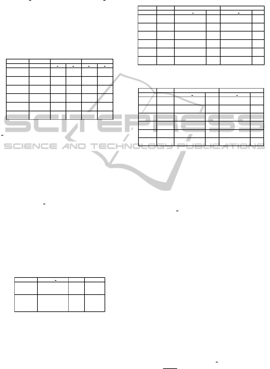
We tested our approach on real-life instances of
CALMA-project (CALMA-website, 1995). The set
of instances consists in two parts. The CELAR in-
stances are real-life problems from a military appli-
cation. The GRAPH instances are randomly gener-
ated problems. We only use the so-called MI-FAP in-
stances (Table 1). In this paper we are only concerned
by instances 6, 7 and 8 of CELLAR and instances 5,
6, 11 and 13 of GRAPH. Other instances were not
considered because they are easy.
Table 1: Benchmark characteristics.
Instance Original graph Reduced graph Best cost
|V| |E| |V| |E|
CELAR06 200 1322 100 350 3389
CELAR07 400 2865 200 816 343592
CELAR08 916 5744 458 1655 262
GRAPH05 200 1134 100 416 221
GRAPH06 400 2170 200 843 4123
GRAPH11 680 3757 340 1425 3080
GRAPH13 916 5273 458 1877 10110
6.2 BMCWD vs. BMCCD
This section presents comparativeresults obtained for
BMCWD and BMCCD algorithms by using 2 and
3 clusters. Notice that the instance CELAR08 is
excluded from this test and all tests concerning ap-
proaches based on decomposition because it is al-
ready decomposed in several and unbalanced clusters.
To compare these algorithmswe based on the measure
1
https://romeo1.univ-reims.fr/, University of Champagne-
Ardenne
ICAART2014-InternationalConferenceonAgentsandArtificialIntelligence
482
parameters % cut previously defined, and % Bn cor-
responding to the ratio of boundary nodes resulting
from the decomposition. This last parameter plays
an important role in our tests because our approach
is mainly focused on the number of boundary nodes.
The balance threshold parameter is fixed to 0.8.
Table 2: % of cut and boundary nodes found by BMCWD
and BMCCD with 2 and 3 clusters.
Instance Method k=2 k=3
% cut % Bn % cut % Bn
CELAR06 BMCWD 2.8 30.5 4 43
BMCCD 3.33 17 4.39 22.5
CELAR07 BMCWD 0.002 36.5 0.7 47.25
BMCCD 0.98 5.75 1.12 7.25
GRAPH05 BMCWD 6 54.5 7.1 75
BMCCD 7.85 47 12 61.5
GRAPH06 BMCWD 7.5 53.5 8.9 61.5
BMCCD 7.37 46.25 11.43 74.5
GRAPH11 BMCWD 5 61.76 8.5 75.29
BMCCD 8.86 51.91 11.71 63.38
GRAPH13 BMCWD 7.8 67.36 9.5 69.65
BMCCD 8.76 50.54 12.33 66.37
Table 2 shows that for 2 clusters the parameter
%
cut is low, while for 3 clusters this parameter in-
creases. This is due to the hierarchical nature of our
decomposition algorithm. The number of boundary
nodes varies from instance to another for both algo-
rithms but BMCCD produces less boundary nodes in
general.
6.3 AGA-MI-FAP Alone
In this section, we report the best costs (cost) and
average costs (avg cost) obtained by using AGA-
MI-FAP alone (50 executions). Initial Mutation and
Crossover probabilities are fixed experimentally to 1
and 0.2 respectively, ∆p
m
= ∆p
c
= 0.1, and the popu-
lation size is fixed to 100.
Table 3 shows clearly the efficiency of AGA-
MI-FAP algorithm. Indeed, optimal solutions have
been obtained for the majority of instances and near-
optimal solutions are obtained on the rest.
Table 3: Performance of AGA-MI-FAP.
Instance cost(avg cost) cpu(s) Best cost
CELAR06 3389(3389) 37 3389
CELAR07 343691(343794) 312 343592
CELAR08 262(264) 571 262
GRAPH05 221(221) 35 221
GRAPH06 4124(4128) 222 4123
GRAPH11 3119(3191) 2246 3088
GRAPH13 10392(10812) 3700 10110
6.4 Approaches using Decomposition
In this section we present the results for Top-Down
and Iterative Top-Down on 2 clusters and 3 clusters.
6.4.1 Top-Down Algorithm
Table 5 reports the results obtained with Top-Down
Table 4: Results of Top-Down with 2 and 3 clusters.
Instance Method k=2 k=3
BMC cost(avg cost) cpu cost(avg cost) cpu
CELAR WD 3389(3822) 13 3422(5302) 10
06 CD 3389(3499) 15 3402(4922) 10
CELAR WD 363897(434297) 161 353800(2455320) 74
07 CD 343592(1374412) 120 343912(1385114) 84
GRAPH WD 221(382) 26 267(869) 15
05 CD 221(236) 21 257(844) 14
GRAPH WD 4126(4431) 160 5019(9090) 63
06 CD 4126(4311) 175 4193(7107) 83
GRAPH WD 3466(4038) 763 8779(19983) 310
11 CD 3256(4060) 677 7616(12367) 231
GRAPH WD 11015(14256) 1690 25140(32571) 690
13 CD 10796(12511) 1810 22333(31035) 575
Table 5: Results of Iterative Top-Down with 2 and 3 clus-
ters.
Instance Method k=2 k=3
BMC cost(avg cost) cpu cost(avg cost) cpu
CELAR WD 3401(3873) 20 3420(3820) 19
06 CD 3423(3861) 23 3401(4067) 20
CELAR WD 425218(1476655) 219 424126(1353999) 153
07 CD 343810(536322) 179 343691(444117) 164
GRAPH WD 255(391) 21 238(1897) 18
05 CD 221(345) 25 225(643) 20
GRAPH WD 4340(7810) 169 4861(8084) 151
06 CD 4298(5631) 147 4632(6569) 161
GRAPH WD 4119(7500) 751 4127(9751) 551
11 CD 4195(7182) 892 3673(7490) 632
GRAPH WD 17183(19495) 1998 19846(26701) 1456
13 CD 13278(18757) 1969 17255(25885) 1501
algorithm on 2 and 3 clusters. The quality of solutions
of Top-Down algorithm decreases when the number
of clusters increases. This is due to the increasing ra-
tio of boundary nodes leading to a search space reduc-
tion . We also observe that generally the results ob-
tained using Top-Down algorithm based on BMCCD
algorithm are better than those obtained by using BM-
CWD. This is due to the same observation made about
the parameter % cut .
6.4.2 Iterative Top-Down Algorithm
Table 4 reports results obtained by Iterative Top-
Down algorithm for 2 and 3 clusters. The populations
size considered is 30 and number of iterations is fixed
to 10. In general larger the population is better is the
solution. The results obtained by Iterative Top-Down
algorithm are encouraging and clearly improves the
simple Top-Down algorithm (k=3). In general, Iter-
ative algorithm maintains its performance even when
the number of clusters increases, while the execution
time decreases. The performance of the simple Top-
Down algorithm decreases considerably with increas-
ing number of clusters while the Iterative Top-Down
one is much more stable.
6.5 Direct vs. Decomposition
Table 6 summarizes the results obtained by direct al-
gorithm and best results obtained by approaches via
decomposition. The parameter σ
cpu is the speed-up
defined as
|CPU1|
CPU2
, where CPU1 and CPU2 are the ex-
DecompositionTehniquesforSolvingFrequencyAssigmentProblems(FAP)-ATop-DownApproach
483
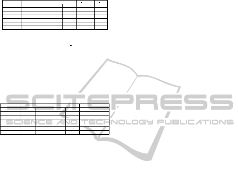
Table 6: Comparing direct and decomposition approaches.
Instance Direct Via decomposition σ cost(%) σ cpu
cost cpu cost cpu
CELAR06 3389 37 3389 13 0.00 2.84
CELAR07 343691 312 343592 120 -0.02 2.60
GRAPH05 221 35 221 21 0.00 1.66
GRAPH06 4124 222 4126 160 0.04 1.38
GRAPH11 3119 1946 3256 677 4.39 2.87
GRAPH13 10392 3700 10796 1810 3.88 2.04
ecution times of direct approach and that via decom-
position respectively . The row σ
cost shows clearly
that the results are comparable with the quality of the
solutions on all instances. However, the row σ
cpu
outlines clearly the benefit of approaches via decom-
position in term of cpu time. this corresponds to our
first objective aiming to solve large problems in short
time near to optimality.
Table 7: Comparison with recent decomposition algo-
rithms.
Instance Our approach All 10 Fon 13
cost cpu(s) cost cpu(s) cost cpu(s)
CELAR06 3389 13 3389 212 3389 93
CELAR07 343592 120 343592 607 343592 317
GRAPH05 221 21 - - 221 10
GRAPH06 4126 160 - - 4123 240
GRAPH11 3256 677 - - 3080 2762
GRAPH13 10796 1810 - - 10110 3196
6.6 Comparison with Related Works
Table 7 compare the best results we obtained by our
algorithms based on decomposition and the best re-
sults of (Allouche et al., 2010) and (Fontaine et al.,
2013)) which both exploit Tree Decomposition of
problems to be solved.
Our results are comparable to those presented in
(Fontaine et al., 2013) in terms of quality of the solu-
tion but are better in terms of CPU-time.
7 CONCLUSIONS
In this paper, a Top-Down approach is developed for
solving hard instances of MI-FAP problem near to op-
timality in short time.
To validate experimentally this approach:
• Two decomposition methods based on a Min-Cut
algorithm were implemented. The first one called
BMCWD aims to minimize the global weight of
the cut. The second one called BMCCD aims to
minimize the number of edges of the cut.
• An adaptive genetic algorithm (AGA-MI-FAP)
was proposed to solve the initial problem without
decomposition or for solving the sub-problems.
• The 1-opt local search heuristic was used to im-
prove the global solution.
The quality of the solutions and the runtime of the
different approaches, with and without decomposi-
tion, were compared on instances of CALMA project.
Almost instances were solved using AGA-MI-FAP.
When solving decomposed MI-FAP, optimal or near-
optimal solutions were obtained in a short time with
the proposed method. The Iterative Top-Down algo-
rithm have good performances even when the number
of clusters increases. This promising result leads to
investigate further this decomposition approach. The
first results obtained in this work indicate that the best
strategy proposed can significantly improve the com-
putation time without any significant loss of quality
of the solution.
Several perspectives to this work will be investi-
gated: different decomposition methods and criteria,
other exact or heuristic algorithms to solve the clus-
ters.
REFERENCES
Aardal, K., Van Hoessel, S., Koster, A., Mannino, C., and
Sassano, A. (2003). Models and solution techniques
for frequency assignment problems. 4OR, Quaterly
Journal of the Belgian, French and Italian Operations
Research Sciences, 1:261–317.
Allouche, D., Givry, S., and Schiex, T. (2010). Towards
parallel non serial dynamic programming for solving
hard weighted csp. In Proc. CP’2010, pages 53–60.
CALMA-website (1995). Euclid Calma project.
ftp://ftp.win.tue.nl/pub/techreports/CALMA/.
Colombo, G. and Allen, S. M. (2007). Problem decomposi-
tion for minimum interference frequency assignment.
In Proc. of the IEEE Congress in and Evolutionary
Computation, Singapor.
Fontaine, M., Loudni, M., and Boizumault, S. (2013).
Exploiting tree decomposition for guiding neighbor-
hoods exploration for vns. RAIRO-Operations Re-
search, 47/2:91–123.
Hale, W. K. (1980). Frequency assignment: Theory and
applications. 68/12:1497–1514.
Kolen, A. (2007). A genetic algorithm for the partial bi-
nary constraint satisfaction problem: an application
to a frequency assignment problem. Statistica Neer-
landica, 61/1:4–15.
Koster, A., Van Hoessel, S., and Kolen, A. (1998). The par-
tial constraint satisfaction problems: Facets and lifting
theorem. O. R. Letters, 23(3-5):89–97.
Maniezzo, V. and Carbonaro, A. (2000). An ants heuristic
for the frequency assignment problem. Computer and
Information Science, 16:259–288.
Stoer, M. and Wagner, F. (1997). A simple min-cut algo-
rithm. Journal of the ACM, 44/4:585–591.
Voudouris, C. and Tsang, E. (1995). Partial constraint sat-
isfaction problems and guided local search. Technical
report, Department of Computer Science,University
of Essex. Technical Report CSM-25.
ICAART2014-InternationalConferenceonAgentsandArtificialIntelligence
484
