
To Calibrate & Validate an Agent-based Simulation Model
An Application of the Combination Framework of BI Solution &
Multi-agent Platform
Thai Minh Truong
1,2
, Frédéric Amblard
1
, Benoit Gaudou
1
and Christophe Sibertin Blanc
1
1
UMR 5505 CNRS-IRIT, Université Toulouse 1 Capitole, Toulouse, France
2
CIT, Can Tho University, Can Tho, Vietnam
Keywords: Calibration, Validation, BI Solution, Data Warehouse, Multi-Agent Simulation, Agent-based Model, Brown
Plant Hopper.
Abstract: Integrated environmental modeling approaches, especially the agent-based modeling one, are increasingly
used in large-scale decision support systems. A major consequence of this trend is the manipulation and
generation of huge amount of data in simulations, which must be efficiently managed. Furthermore,
calibration and validation are also challenges for Agent-Based Modelling and Simulation (ABMS)
approaches when the model has to work with integrated systems involving high volumes of input/output
data. In this paper, we propose a calibration and validation approach for an agent-based model, using a
Combination Framework of Business intelligence solution and Multi-agent platform (CFBM). The CFBM is
a logical framework dedicated to the management of the input and output data in simulations, as well as the
corresponding empirical datasets in an integrated way. The calibration and validation of Brown Plant
Hopper Prediction model are presented and used throughout the paper as a case study to illustrate the way
CFBM manages the data used and generated during the life-cycle of simulation and validation.
1 INTRODUCTION
Integrated socio-environmental modeling in general
and multi-agent based simulation approach applied
to socio-environmental systems in particular are
increasingly used as decision-support systems in
order to design, evaluate and plan public policies
linked to the management of natural resources
(Laniak et al., 2013). For example, in the research
about invasions of Brown Plant Hopper (BPH) and
the impact of BPH on rice fields of the Mekong
Delta region (Vietnam), researchers must develop
and integrate several models (e.g. BPH growth
model, light-trap model, BPH migration model).
They must also integrate data from different data
sources and analyze the integrated data at different
scales. Such an integrated simulation system
involving high volume of data raises two problems:
how to manage and analyze outputs of simulation
models considering such a high volume of input?
Although computing power is increasing rapidly,
to determine the accuracy of the simulation outputs
from a large size of inputs with several parameters
and to work on the high computational requirements
in large systems are still the limitations of agent-
based modelling (Crooks and Heppenstall, 2012).
When developing a simulation model, the modelers'
ambition is to achieve a credible model. To obtain a
credible model or to determine the accuracy of the
simulation outputs, calibration and validation are
two necessary processes (Donigian, 2002; Klügl,
2008; Law, 2009). For instance, complex agent-
based models are usually executed with several
parameters and generate a huge amount of data,
which do not have exactly the same structure than
observation data from real system and can be
measured and validated in various conditions. In
such case, calibration and validation are used to
determine which inputs and outputs are appropriate
regarding observation data (Ngo and See, 2012;
Rogers and Tessin, 2004; Said et al., 2002).
Furthermore, calibration and validation are among
the greatest challenges in agent-based modelling
(Crooks et al., 2008; Crooks and Heppenstall, 2012).
Therefore, how to solve the two challenges
(calibration and validation) of agent-based
modelling and simulation when the model deals with
172
Minh Truong T., Amblard F., Gaudou B. and Sibertin Blanc C..
To Calibrate & Validate an Agent-based Simulation Model - An Application of the Combination Framework of BI Solution & Multi-agent Platform .
DOI: 10.5220/0004820401720183
In Proceedings of the 6th International Conference on Agents and Artificial Intelligence (ICAART-2014), pages 172-183
ISBN: 978-989-758-016-1
Copyright
c
2014 SCITEPRESS (Science and Technology Publications, Lda.)

integrated systems with a high volume of
input/output data?
In this article, we briefly describe a Combination
Framework of BI solution and Multi-agent platform
(CFBM). CFBM was designed and implemented in
GAMA (Truong et al., 2013) and it can be used to
model and execute agent-based simulation models,
to handle data input/output of the models, and to
conduct data analysis. Subsequently, we expose an
approach for the calibration and validation of multi-
agent models by applying the CFBM, which
proposes a solution to two of the limitations of
agent-based modelling when working in integrated
systems. In addition, a specific measure is presented,
i.e. Jaccard index for ordered data sets, which has
been used to evaluate the accuracy of simulation
outputs.
Hence the major contribution of this article is to
propose an implemented framework (CFBM) to
address two crucial issues in agent-based simulation
that are the calibration and validation of such
models. In order to demonstrate the feasibility and
the interest of the application of such framework, we
apply it to the calibration and validation of a Brown
Plant Hoppe invasion model, which is described
briefly.
In the following sections, we first present the
state of the art of works linking ABMS, BI and
calibration and validation of simulation models
(Section 2). The global architecture of the
Combination Framework of BI solution and Multi-
agent platform is presented in Section 3. In Section
4, we illustrate the calibration and validation
approach for integrated agent-based simulation
models. In Section 5, we apply the approach on an
integrated simulation model, namely the BPH
prediction model, in order to calibrate and validate
the model on the GAMA simulation platform in
order to illustrate the approach. Discussion and
perspectives conclude this article.
2 RELATED WORKS
2.1 Integration of BI Solution into a
Simulation System
Data Warehouse (DW) and analysis tools such as BI
solutions can help users to manage a large amount of
simulation data and to make several data analyses
that support the decision-making processes (Inmon,
2005; Kimball and Ross, 2002). The combination of
simulation tools and DW is on the increase and
being applied in different areas. For example,
although (Madeira et al., 2003; Sosnowski et al.,
2007) are only two applications of OLAP
technologies to a specific problem, these works
demonstrate that a multidimensional database is
suitable to store several hundreds of thousands of
simulation results. Simulation models, DW and
analysis tools with OLAP technologies were also
integrated in decision support systems or forecast
systems (Ehmke et al., 2011; Vasilakis et al., 2008).
In (Mahboubi et al., 2010), Mahboubi et al. also
used data warehouse and OLAP technologies to
store and analyze a huge amount of output data
generated by the coupling of complex simulation
models such as biological, meteorological and so on.
In particular, the authors proposed DW and Online
Analytical Processing tool (OLAP tool) for storing
and analyzing simulation results.
The mentioned state of the art demonstrates
therefore the practical possibility and the usefulness
of the combination of simulation, data warehouse
and OLAP technologies. It also shows the potential
of a general framework that has, as far as we know,
not yet been proposed in the literature.
2.2 Calibration and Validation
What are calibration and validation? The calibration
process is known as a test of a model with known
input and output information. It is used to adjust or
estimate factors for data which are not available. The
validation process is the comparison of model results
with numerical data independently derived from
experiments or observations of the environment.
These two definitions are taken from (Donigian,
2002) who was citing (ASTM, 1984). In the
validation of multi-agent simulation, there are two
kinds of validation: internal validation and external
validation (Amblard et al., 2007). These two
processes are also presented in terms of "face
validation" and "statistical validation" by (Klügl,
2008). Internal validation is used to check the
conformity between specifications and the
implemented model. In the software engineering
field, it is usually called verification and corresponds
to the process which is used to compare the
conceptual model to the computer-generated model.
Internal validation corresponds to building the
model right. External validation is used to check the
similarities between the model and the real
phenomenon. It is also named validation process in
software engineering, so external validation
corresponds to build the right model. In this paper,
we address only the external validation. In the
following, validation then means external validation
ToCalibrate&ValidateanAgent-basedSimulationModel-AnApplicationoftheCombinationFrameworkofBISolution
&Multi-agentPlatform
173
of multi-agent models; and the calibration is the
fine-tuning of the output of simulation model by a
change in the values of parameters. The calibration
involves the validation (especially the similarity
evaluation which is present in both cases) to check
the simulation outputs.
To calibrate and validate a simulation model,
modelers used several different methods: (Donigian,
2002) used the "weight of evidence"; (Ngo and See,
2012; Rogers and Tessin, 2004; Said et al., 2002)
used generic algorithms to optimize the fitness value
of parameters by comparison with the observations
from real systems. In general, these researchers
validate simulation outputs with empirical data and
check fitness conditions by statistic methods such as
Root Mean Squared Error (RMSE) (Ngo and See,
2012; Willmott et al., 1985). Implementing
calibration and validation model in Section 5, we
tune values of parameters in their value domain
(they were specified by expert biologist) by
specifying the different values of all parameters and
execute simulations with all possible cases (full
experimental design in statistical terms). The Jaccard
index (Jaccard, 1908), which can be found in
(Niwattanakul et al., 2013; Rahman et al., 2010;
Sachdeva et al., 2009) is used to estimate the
similarity coefficient between two data sets.
3 COMBINATION FRAMEWORK
OF BUSINESS INTELLIGENCE
SOLUTION AND
MULTI-AGENT PLATFORM
(CFBM)
In this section, we demonstrate the logical
framework to combine BI solution and Multi-agent
platform. This framework has been implemented on
the GAMA simulation platform (Truong et al.,
2013). The CFBM is designed to handle big data
from different data sources and perform analyses on
the integrated data from these sources. It is a
solution to improve the weaknesses of ABMs when
modelling is conducted on an integrated system. In
this framework, we use a BI solution as a database
tool, a multi-agent platform as model design tool and
model execution tool. For the execution analysis
tool, we can either use OLAP analysis tool or use
analysis features of the platform (implemented as an
external plug-in for the platform, e.g. R scripts).
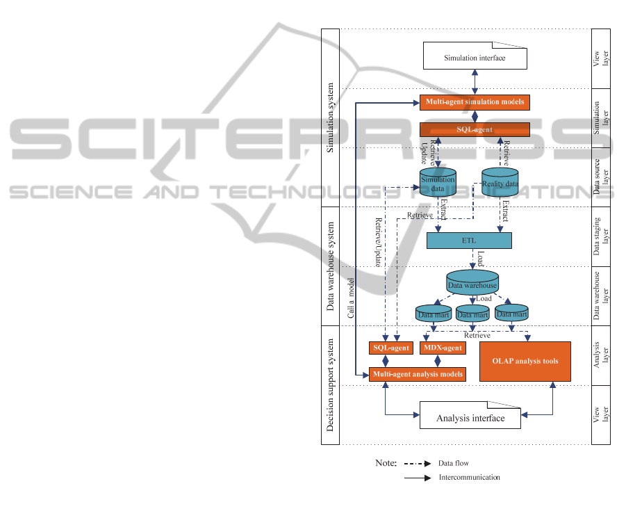
The architecture of the CFBM is illustrated in
Figure 1. It is formed by three systems and it
supports four tools: model design tool, model
execution tool, execution analysis tool and database
tool.
3.1 Simulation System
The simulation system plays two roles: model design
tool and model execution tool. It is composed of a
multi-agent platform and a relational database. This
system is an Online Transaction Processing (OLTP)
or an operational source system. It is an outside part
of the data warehouse (Kimball and Ross, 2002).
Figure 1: Combination framework of BI solution and
multi-agent platform architecture.
Three layers with five components compose the
simulation system. The simulation interface is the
user environment that helps the modeler to design
and implement his models, execute the models and
visualize results. Multi-agent simulation models
are a set of multi-agent based models. They are used
to simulate the phenomena that the modeler aims at
studying. The SQL-agent plays the role of the
database tool and can access to the relational
database. It is a particular kind of agent that supports
Structured Query Language (SQL) functions to
ICAART2014-InternationalConferenceonAgentsandArtificialIntelligence
174

retrieve simulation inputs from simulation data or
reality data, to store output simulation data into
simulation data databases and to transform data (in
particular the data type) from simulation model to
relational database, and conversely. Reality data and
Simulation data are relational databases. The reality
database is used to store empirical data gathered
from the target system that are needed for the
simulation and analysis phases. Finally, Simulation
data is used to manage simulation models,
simulation scenarios and the output results of the
simulation models. These two data sources will be
used to feed the second part of the framework,
namely the Data warehouse system
The simulation system helps to implement
models, execute simulations and handle their
input/output data.
3.2 Data Warehouse System
The data warehouse system is conceptualized as a
part of the BI solution. It is an important part to
integrate data from different sources (simulation
data, empirical data and others external data) and is
used as data storage to feed data for decision support
systems.
The data warehouse system is divided into three
parts. ETL (Extract-Transform-Load) is a set of
processes with three responsibilities. First, it extracts
all kind of data (empirical data and simulation data)
from the simulation system. Second, ETL transfers
the extracted data into an appropriate data format.
Finally, it loads the transferred data into a data
warehouse. Data warehouse is used to store
historical data, which are loaded from simulation
system by ETL. Data mart is a subset of data stored
in the data warehouse and it is a data source for
concrete analysis requirements. We can create
several data marts depending on our analysis
requirements. Data mart is a multidimensional
database, which is designed based on
multidimensional approach. It uses star joins, fact
tables and dimension tables to present the data mart
structure data. With a multidimensional structure,
data mart is particularly useful in improving the
performance of analytic processes.
3.3 Decision Support System
In CFBM, the decision support system plays the role
of analysis tool. It is a software environment
supporting analysis, decision-making features and
the visualization of results. In our design, we
propose to use existing OLAP analysis tools, or a
multi-agent platform with analysis features or a
combination of both options. The decision support
system of CFBM is built on four parts. Analysis
interface is a user interface used to handle analysis
models and visualize results. Multi-agent analysis
models are a set of agent-based analysis models.
They are created based on analysis requirements and
handled via analysis interface. MDX-agent is a
bridge between multi-agent analysis models and data
marts. This agent supports MultiDimensional
eXpressions (MDX) functions to query data from a
multidimensional database. OLAP analysis tools
are analysis software packages that support OLAP
operators.
In general, the CFBM is a solution we proposed
to solve the limitations of ABMS in terms of data
management and output analysis with high volume
of data, which have been explained in Section 1.
The key points of the CFBM architecture are that
it contains and adapts the four features of a computer
simulation system (model design, model execution,
execution analysis, and database management). All
these functions are integrated into one multi-agent
platform. The data warehouse manages the related
data. The analysis models and simulation models
can interact with each other. Using the CFBM
architecture, we can build a simulation system not
only suitable for modeling driven approach but also
for data driven approaches. Furthermore, CFBM
brings certain benefits for building simulation
system with complex requirements such as the
integration and analyzes of high volume of data.
4 CALIBRATION & VALIDATION
APPROACH
In this section, we propose an approach to calibrate
and validate an agent-based simulation model. The
approach is an application of CFBM, which we
presented in Section 3. It is useful when we work
with integrated simulation systems, where we need
to control several models with high volume of
input/output data of simulation, observation data
from real system and analysis results. In this part we
detail the practical use of CFBM to calibration and
validation purposes.
4.1 Calibrating an Agent-based Model
In Figure 2, we present an automatic approach with
seven steps for calibrating and validating an agent-
based model. The approach helps modelers to test
their models more systematically in a given
ToCalibrate&ValidateanAgent-basedSimulationModel-AnApplicationoftheCombinationFrameworkofBISolution
&Multi-agentPlatform
175

parameter space, to evaluate (validate) outputs of
each simulation and manage all data in an automatic
manner.
Step 1: Load input Data with Default Parameter
Values. Select a model scenario from the database
then the input data and default parameter values are
loaded from the quartet (model, scenario, input data
set, parameters). This step assures that the correct
input data and default values of parameter are loaded
to simulation model.
Step 2: Execute Simulation Model. The simulation
model is executed with the loaded scenario as input.
In this process, outputs of the simulation are stored
into a database. Because the simulation can be
executed many times (replications) with the same
scenario, to be sure that the system can handle
results, the quartet (model, scenario, replicate,
output) must be stored into the database.
Step 3: Execute Validation Model. The validation
model is used to analyze the variations between
simulation outputs and observations from the real
system. The result of this process is a similarity
coefficient or difference/distance coefficient
between the output data in step 2 and observation
data. The method is used to validate depends on the
properties of data and on the modeler's choice. For
example, we choose Jaccard index method for the
validation of our model in Section 4.
In this step, the validation model loads testing
data set (observations) and corresponding output
data set of the quartet (model, scenario, replicate,
output) to make the comparison between the two
data sets. The result of validation is also stored into
the database with the quartet (model, scenario,
replicate, result of validation).
Step 4: Check Fitness Condition. The result of
validation in Step 3 is compared with a fitness
condition that is defined by the modeler. For
example, the similarity coefficient of Step 3 must be
greater than or equal to 0.90 (see Section 5.2.1).
There are two cases:
If the fitness is true/yes then do Step 5 (It means
that the input of simulation with the value of the
parameters is accepted).
If the fitness is false/no then do Step 6 (It means
that the input of simulation with the value of the
parameters is not accepted).
Step 5: Store the Scenario with Fitness
Parameters. Note that the result of each replication
was stored in the quartet (model, scenario, replicate,
result of validation) by step 3. Hence this step only
stores the adaptive scenario and fitness parameter
values in the quartet (model, scenario, replicate,
fitness parameter values).
Step 6: Check Adjustment Condition. The system
checks if there is another instance of parameters in
its population or not. Hence there are two cases:
If the Adjustment is True/Yes then do Step 7 (It
means that there is another instance of
parameters in its population).
If the Adjustment is False/No then stopping the
process (It means that there is not any other
instance of parameters in its population).
Step 7: Execute Adjustment Parameters. The
adjustment function concerns the determination of
the new values for parameters. It is used to adjust the
input parameters to improve the output of the model.
The result of this process is the creation of a new
scenario for the simulation model.
This function changes the values of the
parameters to other values in their population and
progresses to step 2.
With the seven-step approach, the calibration
model can execute the simulation model with all
adjusted values of the parameters, manage the whole
input/output data dealt within the processes and
analyze the variant between simulation outputs and
observation data. It helps us to specify appropriate
values of parameters automatically. The calibration
model is an integration of two major models:
simulation model and validation model. It also
handles all data processed by the two models. The
calibration model is a demonstration of the
application of the CFBM, where: BI solution is used
to handle all input/output of the model and empirical
data related with simulating and analyzing while the
analysis model is used to validate the output of the
simulations.
4.2 Validating Simulation Output using
Jaccard Index
There are several methods to measure similarity
between two data sets as mentioned in (Ngo and
See, 2012; Wolda, 1981). Root Mean Squared Error
(RMSE) is usually used to estimate the distance (or
error) between two data sets (simulation outputs and
observations from real system).
ICAART2014-InternationalConferenceonAgentsandArtificialIntelligence
176
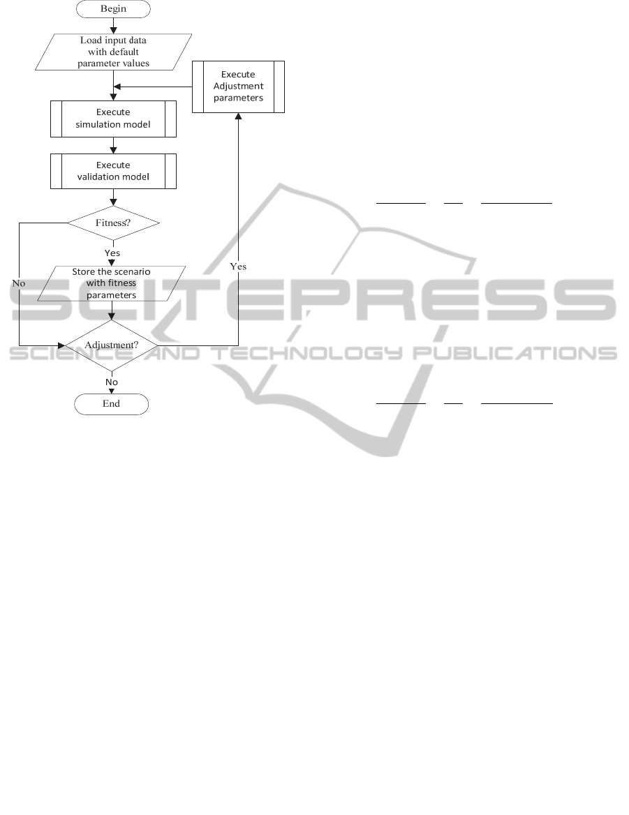
Figure 2: Workflow for the calibration of a model.
In this section, we propose a method to measure
the similarity between two data sets integrating
constraints on the position of elements in the data
sets (ordered data set). In our method, we use
Jaccard index as the similarity coefficient between
two ordered data sets as follow:
Jaccard Index on Ordered Data Sets. Assume that
we have two ordered data sets:
X = {x
1
, x
2
, …., x
n
}
Y = {y
1
, y
2
, …., y
n
}
Definition 1: x
i
is called match (or similar or equal)
with y
j
when i = j and value of x
i
equal value of y
j
.
match(x
i
, y
j
) = true when i = j and
value(x
i
) = value(y
j
) other match(x
i
, y
j
) = false
i,j=1..n
(1)
Definition 2: The intersection of X and Y is:
S={s
1
, s
2
, …, s
n
} (2)
where:
s
i
= {x
i
} (or s
i
= {y
i
}) when match(x
i
,y
j
) = true
s
i
= {} = ∅ when match(x
i
, y
j
) = false
i=1..n
Definition 3: The union of X and Y is:
U={u
1
, u
2
, …, u
n
} (3)
where:
u
i
= {x
i
} (or u
i
= {y
i
}) when match(x
i
,y
j
) = true
u
i
= {x
i
, y
i
} when match(x
i
, y
j
) = false
i =1..n
Definition 4: The cardinality of an ordered set is
| {} |=0;
| S |=| s
1
| + | s
2
| + … + | s
n
|
| U |=| u
1
| + | u
2
| + … + | u
n
| = | X |+| Y | - | S |
(4)
Definition 5: Jaccard index of two ordered data sets
is:
J
,
∩
∪
|
|
|
|
(5)
where:
c: number of matched pairs (xi, yi)
a: number of x
i
elements in X and not matched y
i
in Y
b: number of y
i
elements in Y and not matched x
i
in X
In an easier way, we calculate Jaccard index
between X and Y based on the cardinality of S, X and
Y as equation (6):
J
,
∩
∪
|
|
|
|
(6)
where:
f: cardinality of S.
d: cardinality of X.
e: cardinality of Y.
Example 1: Assume that we have the following
data:
Empirical data set: X={ 1,2,3,4,5}
Simulation data set: Y={ 3,2,5,6,7}
Jaccard index between X and Y with no constraint on
position of elements:
Intersect(X, Y) = {2, 3, 5}
Union(X, Y) = {1, 2, 3, 4, 5, 6, 7}
J(X, Y) = 3/(2+2+3) = 3/7 = 0.429
However we cannot say x
3
=y
1
because we consider
ordered sets. In this case, we apply Jaccard index on
two ordered data sets:
Intersect(X, Y) = { {}, {2}, {}, {}, {} }
Union(X, Y) = { {1,3}, {2}, {3,5}, {4,6}, {5,7} }
(5) => J(X, Y) = 1/(4+4+1) = 1/9 = 0.111 or (6) =>
J(X, Y) = 1/(5+5-1) = 1/9 = 0.111
In Example 1, the similarity coefficient (Jaccard
index) between two data sets with no position
constraint (0.429) is different from the similarity
coefficient between those two data sets with position
constraint (0.111).
ToCalibrate&ValidateanAgent-basedSimulationModel-AnApplicationoftheCombinationFrameworkofBISolution
&Multi-agentPlatform
177

5 CALIBRATION & VALIDATION
OF THE BPH PREDICTION
MODEL
In this section, we demonstrate the calibration and
validation model for an integrated agent-based
simulation model, the BPH prediction model
(Truong et al., 2013). This model is one of the
research results of the DREAM
1
project, coordinated
between Can Tho University, Vietnam and Institut
de Recherche pour le Développement (IRD), France.
5.1 BPH Prediction Model
BPH Prediction model is used to predict the Brown
Plant Hopper (cricket) density on rice fields in
Mekong Delta, Vietnam. This model contains two
sub-models: BPH Growth Model and BPH
Migration Model. The output is the number of BPHs
in each light-trap distributed in the environment to
catch BPH. Inputs and outputs of the integrated
model are handled via the CFBM in GAMA.
Empirical data such as administrative boundary
(region, river, sea region, land used), light-trap
coordinates, daily trap-densities, rice cultivated
regions, general weather data (wind data), station
weather data (temperature, humidity, etc.), river and
sea regions are used as inputs of the simulation
model and as validation data for the model.
5.1.1 BPH Migration Model
BPH migration model is used to simulate the
invasion of BPHs on the rice fields. The migration
process of BPHs in the studied region is modeled by
a dynamical moving process on cellular automata.
Denoting x(t) as the number of adult BPHs at
time t, the migration model essentially determines
the outcome x
out
(t) at a later time t + 1 from a
specific source cell and the rates of x
out
(t) moving to
all destinations at time (t + 1). Destination cells are
determined by the semi-circle under the wind, while
the radius of the circle is determined by the wind
velocity and the migration time in a day. The local
constraints are also considered by two combinational
indices: attractiveness index and obstruction index (
(Truong et al., 2013).
1
http://www.ctu.edu.vn/dream/
5.1.2 BPH Growth Model
In the growth model, authors applied a deterministic
model of T variables where T is the life cycle of the
insect. To simplify the implementation process,
these variables will be stored in an array variable V
of length T where an element V[i] marks the number
of insects at age i (i.e. i
th
day of BPH life cycle). For
each simulation step, all elements of V will be
updated by the following equation:
∗
∗,1
∈
1
∗
∗,∈
1
∗
∗,∈
1
∗, ∈
(7)
where
denotes the number of insects at age i,
denotes the ratio of egg number able to
become the nymph,
denotes the ratio of nymph number able to
become the adult.
denotes the ratio of eggs can be produced by
an adult.
m denotes the ratio of natural mortality.
denotes the egg giving time span.
denotes the egg and time span.
denotes the nymph time span.
denotes the adult time span.
5.2 Calibration & Validation of the
BPH Prediction Model
5.2.1 Parameters for Calibration
From equation (7) in Section 5.1.2, there are several
parameters we can choose for calibration. However,
we only choose T
4
(adult time span of BPH) and m
(the ratio of natural mortality) as two parameters for
demonstration purpose. BPH has an adult time span
of 8 days in minimum and 12 days in maximum. The
ratio of natural mortality is 0.15 in minimum and
0.35 in maximum. The following populations of the
two parameters are therefore tested:
T
4
: [8, 9, 10, 11, 12]
m=[0.35, 0.25, 0.15]
For the input data of BPH prediction model, we used
the data from 48 light-traps of three typical
provinces in the Mekong Delta region: Soc Trang,
Hau Giang and Bac Lieu from January 1, 2010. With
one input data set, we have 15 scenarios as presented
in Table 1.
ICAART2014-InternationalConferenceonAgentsandArtificialIntelligence
178

Table 1: The parameters value of scenarios for a complete
experimental design.
Scenario
Parameters
Adult time span (T
4
)
Ratio of natural
mortality (m)
1 8 0.35
2 9 0.35
3 10 0.35
4 11 0.35
5 12 0.35
6 8 0.25
7 9 0.25
8 10 0.25
9 11 0.25
10 12 0.25
11 8 0.15
12 9 0.15
13 10 0.15
14 11 0.15
15 12 0.15
The Fitness Condition. We try the fitness condition
in two cases:
Case 1: The difference coefficient is equal or less
than 500
if (RMSE<=500.0)
{
saveFitness(MODEL_ID, SCENARIO_ID,
REPLICATE_ID, PARA_VALUES);
}
Case 1: The similarity coefficient is equal or greater than 0.9
if (Jindex>=0.9)
{
saveFitness(MODEL_ID, SCENARIO_ID,
REPLICATE_ID, PARA_VALUES);
}
saveFitness is a user defined function, it writes
the fitness scenario to database.
5.2.2 Simulation Output and Empirical Data
All related operations for validation in the validation
model are shortly introduced in this part. As
mentioned, the output of BPH prediction model is
the BPH density by light-traps and by time. The
empirical data (testing data) is BPH density from 48
light-traps of three typical provinces in the Mekong
Delta region: Soc Trang, Hau Giang and Bac Lieu
from January 1, 2010.
We simulate and predict the infection of the
BPHs on the rice fields of the three provinces in 28
days. The output of the BPH prediction model has
been structured as in Table 2. The structure of
empirical data is presented in Table 3. Each table
has 48 columns and 28 rows. The columns stand for
48 light-traps and the rows for 28 days (prediction
time). In Table 2, s
i,j
is the number of BPH that is
simulated in step i (day i) at light-trap j. In Table 3,
e
i,j
is the number of BPHs that are caught in day i at
light-trap j on the rice fields of Mekong Delta,
Vietnam. It should be noted that the indices of the
rows and columns starts at 0 for programming
reasons.
Table 2 and Table 3 present two matrixes of
values which have constraints on the position
(location and time) of their elements, hence they are
considered as two ordered data sets.
Table 2: Simulation outputs.
Light-trap
Tr0 Tr1 ... Tr47
day
0 s
0,0
s
0,1
... s
0,47
1 s
1,0
s
1,1
... s
1,47
... ... ... ... ...
27 s
27,0
s
27,1
... s
27,47
Table 3: Empirical data.
Light-trap
Tr0 Tr1 ... Tr47
day
0 e
0,0
e
0,1
... e
0,47
1 e
1,0
e
1,1
... e
1,47
... ... ... ... ...
27 e
27,0
e
27,1
... e
27,47
5.2.3 Validating the Output of the BPH
Prediction Model
The simulation output and testing data have location
constraints (light-trap) and time constraints. Hence,
we use Jaccard index on ordered data sets, which has
been presented in Section 4.2 to estimate the
similarity between the simulation output and the
empirical data. The RMSE method has also been
applied to measure the difference between the two
data sets.
As regard to prediction, we need to predict
different periods of time: from day 0 (initial day) to
6 (1
st
week), from day 7 to 13 (2
nd
week), from day
14 to 20 (3
rd
week) and from day 21 to 27 (4
th
week).
Hence for each scenario, we validate the results of
simulation in four cases: 1
st
week, 2
nd
week, 3
rd
week, 4
th
week. For each case of validation, we
measure difference coefficient (RMSE) and
similarity coefficient (Jaccard index).
In addition, we also measure RMSE and Jaccard
index of the whole data set (from day 0 to 27 or 4
weeks) for the comparison of the two measures in
each scenario.
5.2.3.1 The Difference Coefficient (RMSE)
The difference coefficient between the two data sets
is calculated based on the equation (8):
ToCalibrate&ValidateanAgent-basedSimulationModel-AnApplicationoftheCombinationFrameworkofBISolution
&Multi-agentPlatform
179

∑∑
,
,
∗
(8)
where:
m denotes the number of rows of data set
n denotes the number of columns of data set
e
i,j
is the empirical data. It denotes the number of
BPHs caught in day i at light-trap j.
s
i,j
is the simulation output. It denotes the
number of BPHs obtained in step i (day i) at
light-trap j.
The RMSE results of the 15 scenarios are presented
in Table 4.
Table 4: RMSE between simulation output and empirical
data.
Scenario 1
s
t
week 2
nd
week 3
rd
week 4
th
week 4 weeks
1
483.24 35.53 84.07
1610.25 879.58
2
474.58 31.73 95.14
1714.17 931.34
3
57.17 28.34 119.74
1762.46 928.09
4
53.48 25.71 282.73
1768.57 939.68
5
51.96 19.16 489.3
1738.06 944.39
6
484.26 108.54 209.26
1609.61 885.86
7
472.54 105.35 234.76
1713.14 937.82
8
56.45 106.86 233.00
1761.98 934.39
9
54.63 110.65 345.59
1766.14 945.00
10
84.44 94.69
530.54 1735.76 950.25
11
488.51
1215.93 2413.06 1863.30 1666.85
12
473.80
1271.71 2639.58 2322.33 1903.59
13
83.20
1210.19 2570.50 8826.41 4846.08
14
139.46
1339.62 2636.22 10508.34 5709.14
15 770.65 1150.98 2588.53 11430.14 6174.68
Based on the difference coefficient condition
(RMSE ≤ 500.0) in Section 5.2.1, we can show that:
the RMSE of the first 14 scenarios fits the
calibration conditions for the 1
st
week. , this is also
the case for the first 10 scenarios the 2
nd
week and
the first 9 scenarios the 3
rd
week; but none of the 15
scenarios fits the calibration conditions of the 4
th
week.
5.2.3.2 The Similarity Coefficient (Jaccard
Index)
We apply equation (6) in Section 4.2 to measure the
Jaccard index between the simulation output (Table
2) and empirical data (Table 3). The results are
presented in Table 5.
If we compare the results in Table 5 with the
similarity coefficient condition (Jindex ≥ 0.90) in
Section 5.2.1 then there are not any results fitting the
condition. Certainly, there are no scenarios to be
recognized in the calibration process. This problem
can be explained by the reason that the numbers of
BPHs caught at each light-trap by time has a wide
range of values, from zero to ten thousands. Hence,
to exactly simulate the number of BPHs at each
light-trap over time is impossible or Jaccard index
of two ordered data sets is not suitable to measure
the similarity coefficient between two matrixes of
values where the domain of elements is large. For
this reason, we transformed the number of BPH in
Table 2 and Table 3 to the BPH infection with the
mapping as in Table 6. It means that we change from
the ratio scale to ordinal scale. The scale in Table 6
is proposed by biologists and it was used in (Phan et
al., 2010). The structures of the two transformed
tables are the same as Table 2 and 3, but the value in
each cell ranges from 0 to 4 and its meaning is the
BPH infection level.
Table 5: Jaccard index between simulation output and
empirical data.
Scenario 1
st
week 2
nd
week 3
rd
week 4
th
week 4 weeks
1 0.4071 0.3352 0.2826 0.4573 0.3701
2 0.4525 0.3035 0.2672 0.4382 0.3629
3 0.4651 0.2586 0.2936 0.4015 0.3513
4 0.4547 0.2553 0.3085 0.3682 0.3435
5 0.3952 0.2785 0.3387 0.3490 0.3393
6 0.1845 0.1482 0.1894 0.1362 0.1630
7 0.1799 0.1516 0.1923 0.1267 0.1607
8 0.1647 0.1320 0.2001 0.1147 0.1506
9 0.1580 0.1922 0.1910 0.1136 0.1610
10 0.1560 0.1804 0.1894 0.1040 0.1546
11 0.1580 0.1239 0.1831 0.1317 0.1479
12 0.1554 0.1430 0.1920 0.1120 0.1484
13 0.1728 0.1371 0.1944 0.1196 0.1539
14 0.1346 0.1701 0.1633 0.0993 0.1396
15 0.1313 0.1649 0.1602 0.0915 0.1345
Table 6: Transform BPH density to BPH infection.
Number of BPH BPH Infection Meaning
<500 0 Normal
50 − <1500 1 Light infection
1500 − <3000 2 Medium infection
3000 − ≤10000 3 Heavy infection
>10000 4 Hopper burn
We applied the Jaccard index to measure the
similarity of the two transformed tables and its
results are presented in Table 7.
Based on the similarity coefficient condition
(Jindex ≥ 0.9) in Section 5.2.1, we got the same
scenarios, which are fitted with the difference
coefficient conditions in Section 5.2.3.1.
From the validation results, the calibration model
can choose the scenarios with parameters checking
the specified fitness condition in the calibration
model.
ICAART2014-InternationalConferenceonAgentsandArtificialIntelligence
180
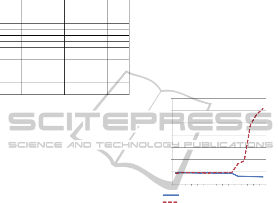
Table 7: Jaccard index on BPH infection data sets.
Scenario 1
s
t
week 2
nd
week 3
rd
week 4
th
week 4 weeks
1
0.9823 1.0000 0.9941
0.7819 0.9293
2
0.9823 1.0000 0.9882
0.7534 0.9187
3
1.0000 1.0000 0.9765
0.7376 0.9147
4
1.0000 1.0000 0.9535
0.7336 0.9082
5
1.0000 1.0000 0.9200
0.7376 0.9016
6
0.9823 0.9862 0.9535
0.7819 0.9169
7
0.9804 0.9882 0.9292
0.7534 0.9021
8
1.0000 0.9882 0.9273
0.7323 0.8990
9
1.0000 0.9862 0.9037
0.7297 0.8922
10
0.9901 0.9862
0.8736 0.7297 0.8828
11
0.9765
0.6649 0.6260 0.4197 0.6396
12
0.9745
0.6622 0.6083 0.3989 0.6265
13
0.9882
0.6583 0.5975 0.3644 0.6121
14
0.9765
0.5975 0.6417 0.3419 0.5979
15 0.8329 0.6970 0.6272 0.3257 0.5863
6 DISCUSSION
Applying CFBM to Calibration and Validation.
There have been many studies, which proposed
frameworks aiming at building credible simulation
models (Law, 2009) in general or at validating agent
based simulation models (Klügl, 2008) in particular.
Although those frameworks instructed us the
processes to archive simulation model with the
accuracy of the simulation output, we still need a
concrete approach to solve two challenges of agent-
based models, which we explained in the
introductory section. By applying CFBM, we
developed a calibration and validation approach for
agent-based models that can help not only to handle
the inputs/outputs of agent-based simulation models
but also to calibrate and validate the agent-based
simulation in an automatic manner. In the Section 4,
we did not demonstrate the concrete method to
adjust the parameters of the simulation model such
as "weight of evidence" (Donigian, 2002) or generic
algorithm (Ngo and See, 2012) because of two
reasons: we only propose the general calibration
approach and adjustment method should be
implemented depending on the case study.
Furthermore, our approach only concerns the
management of the input/output data of simulation
model and validation model and the automation of
the calibration process. They are useful when
working on integrated simulation systems with high
amount of data. For instance, we successfully
applied our approach to calibrate and validate the
BPH prediction model with several data sources
such as administrative boundary (region, river, sea
region, land used), light-trap coordinates, daily trap-
densities, rice cultivated regions, general weather
data (wind data), station weather data (temperature,
humidity, etc.), river and sea regions of three
provinces of Mekong Delta region of Vietnam as we
explained in Section 5. It helped us to reduce time
and work force.
Jaccard Index on ordered Data Sets vs. RMSE. In
experiment, we also compared the Jaccard index on
ordered data sets and RMSE by investigating the
variation of RMSE in Table 4 and Jaccard index of
the two BPH infection tables (the results of the
transformation of Table 2 and 3) in Table 7. For
instance, we compared the values of RMSE on the
whole data sets (column 4 weeks in Table 4) with the
values of Jaccard index (column 4 weeks in Table 7)
by using Graphical method as Figure 3. It should be
noticed that the values of RMSE in Figure 3 were
divided by 1000.
Figure 3: RMSE & Jaccard index on whole data sets.
Figure 3 shows that there is an accordance
between RMSE and Jaccard index. For instance, in
scenario 1, as the RMSE get the lowest value of
879.58, the Jaccard index obtains the highest value,
which is 0.9293. In scenario 11, when the RMSE
suddenly increases to 1666.85, the Jaccard index
decreases to 0.6396 as well. In scenario 15, whereas
RMSE gets the highest value 6174.68, the Jaccard
index gets the lowest value, i.e. 0.5863. It proves
that we can use Jaccard index on ordered data for the
transformed data as fitness condition, which has
been presented in Section 5.2.1.
The Combination on the Fitness Condition. In the
calibration of BPH prediction model, we can choose
RMSE or Jaccard index as a fitness condition.
However, it is suggested to use the combination of
both coefficients, for instance:
if ((Jindex>=0.9) & (RMSE<=100))
{
saveFitness(MODEL_ID, SCENARIO_ID,
REPLICATE_ID, PARA_VALUES);
}
0,0000
1,0000
2,0000
3,0000
4,0000
5,0000
6,0000
7,0000
1 2 3 4 5 6 7 8 9 10 11 12 13 14 15
Value
Scenario
Jindex
RMSE
ToCalibrate&ValidateanAgent-basedSimulationModel-AnApplicationoftheCombinationFrameworkofBISolution
&Multi-agentPlatform
181

The combination of similarity and difference
coefficients helps to have better fitness condition for
choosing the appropriate scenario in calibration.
The Jaccard Index with Aggregation. Assume that
we have two modality matrixes and the domain of
the elements in S and E are [0..k-1], have k values:
,
…
,
…… …
,
…
,
,
…
,
…… …
,
…
,
(9)
The aggregation on the columns on S (or E) has a
matrix:
,
…
,
…… …
,
…
,
(10)
where:
C denotes aggregation matrix on the columns of
matrix S (or E).
c
i,j
is the number of elements in row i in S (or E)
having value j.
The aggregation on the rows on S (or E) has a
matrix:
,
…
,
…… …
,
…
,
(11)
where:
R denotes aggregation matrix on the rows of
matrix S (or E).
r
i,j
is the number of elements at columns j in S (or
E) having the value i.
Then we can apply the Jaccard index on ordered data
sets to the aggregation matrices (equation 10, 11) of
S and E.
7 CONCLUSIONS
In this paper, we introduced a conceptual
framework, which is adapted to multi-agent models
with high volume of data. CFBM supports experts
not only to model a phenomenon and execute the
models via a multi-agent platform, but also to
manage a set of models with their input and output,
to aggregate and analyze the model output data via
data warehouse and OLAP analysis tools.
The key features of CFBM are that it supplies
four components: (1) model design, (2) model
execution, (3) execution analysis and (4) database
management. These components are coupled and
combined in a simulation system. The distinguished
value of CFBM is that it augments the combination
power of data warehouse, OLAP analysis tools and
of a multi-agent based simulation platform. These
components, when put together, are useful to
develop complex simulation systems with a large
amount of input/output data, which can be a what-if
simulation system, a prediction/forecast system or a
decision support system.
In this article, we proposed an automated
calibration approach; it helps modelers to solve the
limitations of ABMs concerning calibration and
validation of agent-based models with high volume
of data: BI solution is used to manage the high
volume of input/output of the simulation models and
the analysis model is used to validate the accuracy of
simulation outputs on large size of input with
varying parameters. We also proposed a specific
method to measure the similarity coefficient of two
data sets with the constraints on the position of
elements, which is called "Jaccard index on the
ordered data sets". In our opinion, the method can
not only be used as a demonstration of validating for
BPH prediction model but it is also a good approach
to validate the output of other models with
constraints on location and time.
Although our calibration and validation approach
is the automation model with the integration of
coupled models (simulation model and validation
model) we have not succeeded in implementing it in
GAMA. For instance, we execute the BPH
prediction model with all values of the parameters
via batch process. Subsequently, we execute the
validation model to validate the outputs and select
appropriate scenarios based on the fitness condition.
These are still two separate processes but not
integrated in one model as designed in Section 4.
This is the problem that we plan to solve in the
future.
As for further work, on one hand we will
continue to develop and improve features for
specific agents (SQL-agent, OLAP-agent and
Analysis-agent) of the CFBM described in Section 3
to GAMA platform. On the other hand, we will also
apply CFBM on multi-scale in multi-agent
simulation or building what-if system, prediction
system and decision support system.
REFERENCES
Amblard, F., Bommel, P., Rouchier, J., 2007. Assessment
and Validation of Multi-agent Models. In: Phan, D.,
ICAART2014-InternationalConferenceonAgentsandArtificialIntelligence
182

Amblard, F. (Eds.), Agent-Based Modelling and
Simulation in The Social and Human Sciences. The
Bardwell Press, Oxford, pp. 93–114.
ASTM, 1984. Standard Practice for Evaluating
Environmental Fate Models of Chemicals. American
Society of Testing Materials. Philadelphia.
Crooks, A., Castle, C., Batty, M., 2008. Key challenges in
agent-based modelling for geo-spatial simulation.
Comput. Environ. Urban Syst. 32, 417–430.
Crooks, A. T., Heppenstall, A. J., 2012. Introduction to
Agent-Based Modeling. In: Heppenstall, A.J., Crooks,
A. T., See, L. M., Batty, M. (Eds.), Agent-Based
Models of Geographical Systems. Springer
Netherlands, Dordrecht, pp. 85–105.
Donigian, A. S., 2002. Watershed model calibration and
validation: The HSPF experience. In: Water
Environment Federation. pp. 44–73.
Ehmke, J. F., Grosshans, D., Mattfeld, D. C., Smith, L. D.,
2011. Interactive analysis of discrete-event logistics
systems with support of a data warehouse. Comput.
Ind. 62, 578–586.
Inmon, W. H., 2005. Building the Data Warehouse, 4th ed.
Wiley Publishing Inc.
Jaccard, P., 1908. Nouvelles recherches sur la distribution
florale. Bull Soc. Vaud. Sci. Nat 223–270.
Kimball, R., Ross, M., 2002. The Data Warehouse
Toolkit: The Complete Guide to Dimensional
Modeling, 2nd ed. John Wiley & Sons, Inc.
Klügl, F., 2008. A validation methodology for agent-based
simulations. In: Proceedings of the 2008 ACM
Symposium on Applied Computing. pp. 39–43.
Laniak, G. F., Rizzoli, A. E., Voinov, A., 2013. Thematic
issue on the future of integrated modeling science and
technology. Environ. Model. Softw. 39, 13–23.
Law, A. M., 2009. How to build valid and credible
simulation models. In: Simulation Conference (WSC),
Proceedings of the 2009 Winter. IEEE, pp. 24–33.
Madeira, H., Costa, J. P., Vieira, M., 2003. The OLAP and
data warehousing approaches for analysis and sharing
of results from dependability evaluation experiments.
In: International Conference on Dependable Systems
and Networks. pp. 86–99.
Mahboubi, H., Faure, T., Bimonte, S., Deffuant, G.,
Chanet, J. P., Pinet, F., 2010. A Multidimensional
Model for Data Warehouses of Simulation Results.
Int. J. Agric. Environ. Inf. Syst. 1, 1–19.
Ngo, T. A., See, L., 2012. Calibration and Validation of
Agent-Based Models of Land Cover Change. In:
Heppenstall, A. J., Crooks, A. T., See, L. M., Batty,
M. (Eds.), Agent-Based Models of Geographical
Systems. Springer Netherlands, pp. 181–197.
Niwattanakul, S., Singthongchai, J., Naenudorn, E.,
Wanapu, S., 2013. Using of Jaccard Coefficient for
Keywords Similarity. In: International
MultiConference of Engineers and Computer
Scientists
. pp. 380–384.
Phan, C. H., Huynh, H. X., Drogoul, A., 2010. An agent-
based approach to the simulation of Brown Plant
Hopper (BPH) invasions in the Mekong Delta. In:
Computing and Communication Technologies,
Research, Innovation, and Vision for the Future
(RIVF), 2010 IEEE RIVF International Conference.
IEEE, pp. 1–6.
Rahman, M., Hassan, M. R., Buyya, R., 2010. Jaccard
Index based availability prediction in enterprise grids.
In: Procedia Computer Science. Elsevier, pp. 2707–2716.
Rogers, A., Tessin, P. von, 2004. Multi-objective
calibration for agent-based models.
Sachdeva, V., Freimuth, D., Mueller, C., 2009. Evaluating
the jaccard-tanimoto index on multi-core architectures.
In: Computational Science–ICCS 2009. Springer
Berlin Heidelberg, pp. 944–953.
Said, L. B., Bouron, T., Drogoul, A., 2002. Agent-based
interaction analysis of consumer behavior. In: The
First International Joint Conference on Autonomous
Agents and Multiagent Systems: Part 1. ACM. pp.
184–190.
Sosnowski, J., Zygulski, P., Gawkowski, P., 2007.
Developing Data Warehouse for Simulation
Experiments. In: Rough Sets and Intelligent Systems
Paradigms. Springer Berlin Heidelberg, pp. 543–552.
Truong, T. M., Truong, V. X., Amblard, F., Drogoul, A.,
Benoit, G., Huynh, H. X., Le, M. N., Sibertin-blanc,
C., 2013. An implementation of framework of
Business Intelligence for Agent-based Simulation. In:
The 4th International Symposium on Information and
Communication Technology (SoICT 2013).
Truong, V. X., Huynh, H. X., Le, M. N., Drogoul, A.,
2013. Optimizing an Environmental Surveillance
Network with Gaussian Process − An optimization
approach by agent-based simulation. In: The Sixth
International KES Conference on Agents and Multi-
Agent Systems – Technologies and Applications (KES
AMSTA 2013). IOS Press, pp. 102–111.
Vasilakis, C., El-Darzi, E., Chountas, P., 2008. A decision
support system for measuring and modelling the multi-
phase nature of patient flow in hospitals. In: Intelligent
Techniques and Tools for Novel System Architectures.
Springer Berlin Heidelberg, pp. 201–217.
Willmott, C. J., Ackleson, S. G., Davis, R. E., Feddema, J.
J., Klink, K. M., Legates, D. R., O’Donnell, J., Rowe,
C. M., 1985. Statistics for the evaluation and
comparison of models. J. Geophys. Res. 90, 8995–
9005.
Wolda, H., 1981. Similarity indices, sample size and
diversity. Oecologia 50.3, 296–302.
ToCalibrate&ValidateanAgent-basedSimulationModel-AnApplicationoftheCombinationFrameworkofBISolution
&Multi-agentPlatform
183
