
Contour-Net
A Model for Tactile Contour-tracing and Shape-recognition
André Frank Krause
1
, Thierry Hoinville
1,2
, Nalin Harischandra
1
and Volker Dürr
1,2
1
Department of Biological Cybernetics, Bielefeld University, Bielefeld, Germany
2
Cognitive Interaction Technology - Centre of Excellence (CITEC), Bielefeld University, Bielefeld, Germany
Keywords:
Tactile Sensor, Contour Tracing, Shape Recognition, Artificial Neural Network.
Abstract:
We propose Contour-Net as a bio-inspired model for rhythmic movement control of a pair of insectoid feelers,
able to successively sample the contour of arbitrarily shaped objects. Initial object contact initiates a smooth
transition from a large-amplitude, low-frequency searching behaviour to a local, small-amplitude and high-
frequency sampling behaviour. Both behavioural states are defined by the parameters of a Hopf Oscillator.
Subsequent contact signals trigger a 180
◦
phase-forwarding of the oscillator, resulting in repeated sampling of
the object. The local sampling behaviour effectively serves as a contour-tracing method with high robustness,
even for complicated shapes. Collected contour data points can be directly fed into an artificial neural network
to classify the shape of an object. Given a sufficiently large training dataset, tactile shape recognition can be
achieved in a position-, orientation- and size-invariant manner. Only minimal pre-processing (normalisation)
of contour data points is required.
1 INTRODUCTION
The tactile sense enables humans and animals to ac-
tively perceive their immediate surrounding through
direct physical contacts with an object (Lee and
Nicholls, 1999). In contrast to vision, direct tactile
sampling of an object allows to ’feel’ object proper-
ties like surface texture, chemical properties, temper-
ature, compliance and humidity, that are hard to ob-
tain otherwise (Lederman and Klatzky, 2009). The
sense of touch is independent of light conditions, and
works equally well night and day. Moreover, the di-
rect contact with an external object yields reliable dis-
tance information (Patanè et al., 2012). Therefore, the
tactile sense plays an important role throughout the
animal kingdom, especially in nocturnal species.
Several insect species, for example the honey bee
(Apis mellifera), the American cockroach (Periplan-
eta americana) and the Indian stick insect (Carau-
sius morosus) have become important model organ-
isms for the study of the sense of touch. Insects carry
a pair of antennae that are densely covered with sen-
sory hairs of different modalities (Staudacher et al.,
2005). Honeybees, for example, show a high con-
centration of tactile hairs at their antennal tip (Esslen
and Kaissling, 1976). Active tactile scanning of sur-
faces allows them to discriminate the micro texture of
flowers (Kevan and Lane, 1985) or artificial gratings
(Erber et al., 1998).
An important constraint of the insect tactile sys-
tem is that antennae essentially are one-dimensional
structures that are incapable of providing a two-
dimensional image “at a glance”. Instead, antennae
need to be moved actively in order to sample infor-
mation from different locations within their working-
range. Active tactile sensing is of particular relevance
in near-range exploration. Many insects actively use
their antennae for obstacle localization, orientation
behaviour, pattern recognition, and even for commu-
nication (Staudacher et al., 2005). Similarly, mam-
mals like cats or rats use active whisker movements
to detect and scan objects in the vicinity of the body.
Insect antennae and mammal whiskers have in-
spired robotic research in the area of tactile sensors.
Early work by Kaneko et al. (1998) describes an arti-
ficial antenna using a flexible beam capable of detect-
ing 3D contact locations and surface properties. Rus-
sell and Wijaya (2003) applied an array of whiskers
that passively scan over an object to recognize its
shape using advanced pre-processing contact-points
and decision trees. In Solomon and Hartmann (2006),
robotic whisker arrays were used to generate 3D spa-
tial representations of the environment and extract ob-
ject shapes. Related work done by Kim and Möller
92
Frank Krause A., Hoinville T., Harischandra N. and Dürr V..
Contour-Net - A Model for Tactile Contour-tracing and Shape-recognition.
DOI: 10.5220/0004821700920101
In Proceedings of the 6th International Conference on Agents and Artificial Intelligence (ICAART-2014), pages 92-101
ISBN: 978-989-758-016-1
Copyright
c
2014 SCITEPRESS (Science and Technology Publications, Lda.)
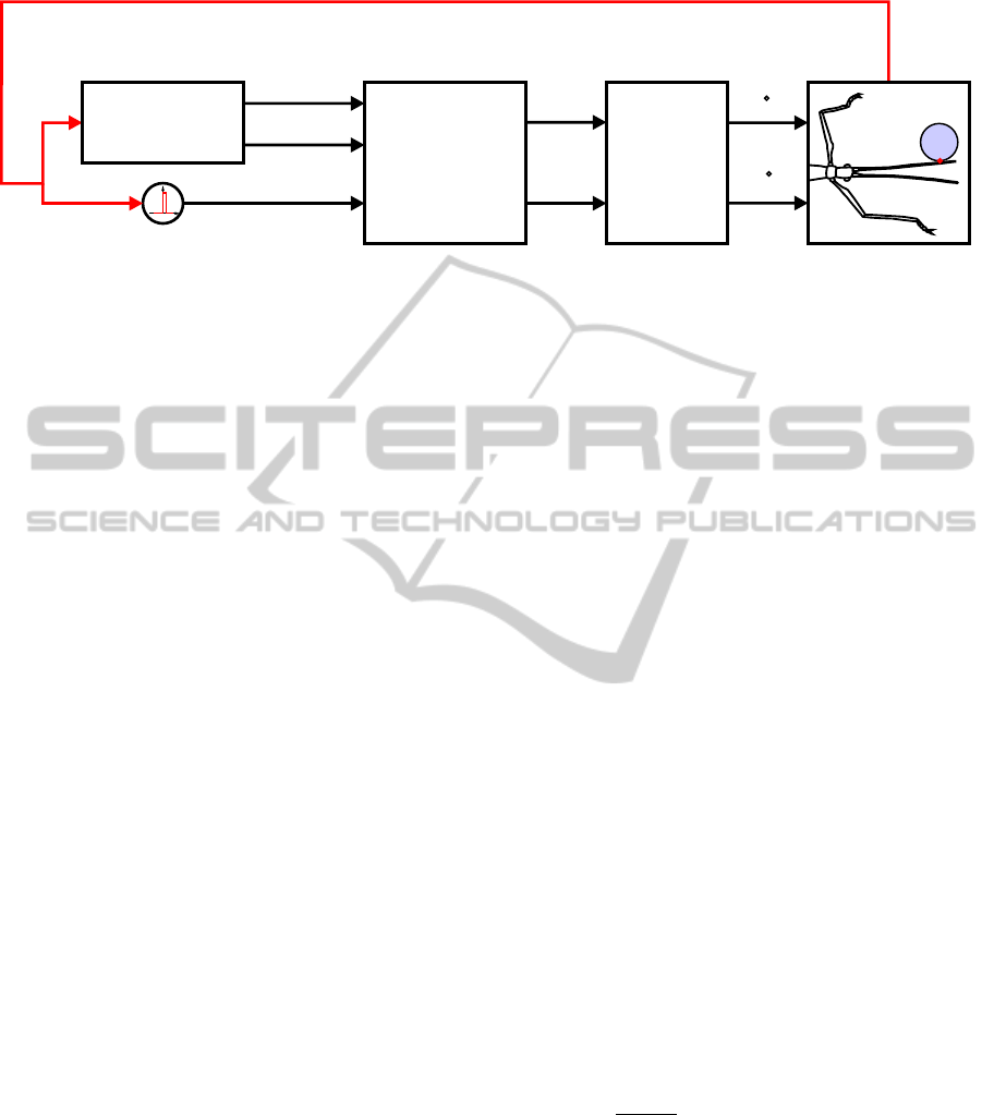
a
b
hopf
oscillator
x
y
+180°
sampling or
searching ?
m
f
contact
scaling
Figure 1: Block diagram of Contour-Net. The binary contact signal (red) determines the frequency and amplitude of the Hopf
Oscillator. The discrete impulse block guarantees that the oscillator phase is forwarded once by 180
◦
, resulting in a movement
away from the object surface. The output of the oscillator is then scaled and drives a simulated or real robot antenna using
velocity control of antennal joints.
(2007) used a vertical whisker array to detect the ver-
tical shape and curvature of objects.
Stick insects continuously and rhythmically move
their antennae during locomotion (Dürr et al., 2001)
and during tactile probing of external objects (Krause
et al., 2013b). Upon antennal contact with an obsta-
cle, stick insects modulate both the frequency and the
amplitude of the rhythmic antennal movement, affect-
ing both antennal joints in a context-dependent man-
ner (Schütz and Dürr, 2011; Krause and Dürr, 2012).
For example, when climbing a square obstacle, they
show a contact-induced switch in behaviour from a
broad, almost elliptical searching pattern to a local
sampling pattern with higher frequency and lower am-
plitude (Krause and Dürr, 2012). This switch to a
local sampling strategy may be interpreted as an ef-
fort to gather more detailed spatial information close
to previous touch locations, effectively leading to the
sampling of an obstacle’s contour.
A fundamental concept explaining such rhythmic
movements in vertebrates and invertebrates is the cen-
tral pattern generator (CPG, for a review see Ijspeert
(2008)). The CPG activity is often modulated by sen-
sory input, proprioceptive input and descending sig-
nals from higher level brain centres. Antennal move-
ments in stick insects are assumed to be driven by
CPGs, because rhythmic activity can be evoked phar-
macologically (Krause et al., 2013b).
Here, we present a simple but effective, bio-
inspired, CPG-based model capturing the essence of
tactile sampling in stick insects. The model is able to
trace the contour of an obstacle using an actively mov-
able tactile probe. The CPG activity is modulated by
a single, binary sensor signal: if the tactile probe is in
contact with the obstacle or not.
2 CONTOUR-NET
The contour-tracing model presented here was coined
Contour-Net, hinting at its possible integration into
existing, modular architectures for simulation and
control of hexapod walking (Walknet, Schilling
et al. (2013)) and ant-inspired navigation (Navi-Net,
Hoinville et al. (2012)). The model captures the es-
sential characteristics of antennal tactile sampling in
stick insects: rhythmic searching movements using
an antenna with two revolute joints with strong cou-
pling and a contact-triggered switch to local sam-
pling. Such rhythmic movements can be obtained as
limit cycles of nonlinear dynamical systems, typically
systems of coupled nonlinear oscillators. In our case
the optimal choice is a “Hopf Oscillator”, because the
two state variables of the oscillator exhibit a fixed
phase coupling and can directly drive the two joints
of an antenna.
2.1 Hopf Oscillator
The Hopf Oscillator is a dynamical system defined
in Cartesian Space by the following differential equa-
tions:
˙x = γ
µ
2
− r
2
x − ωy
˙y = γ
µ
2
− r
2
y + ωx
with r =
p
x
2
+ y
2
. The amplitude of the oscillator
converges to µ, with γ defining the speed of conver-
gence and ω setting the frequency of the limit cycle.
Further, the phase of the oscillator can be set with
x = cos(ϕ), y = sin(ϕ).
The Hopf Oscillator has several advantages: First,
it has a stable limit cycle behavior (i.e., perturba-
tions decay quickly) with a fixed, non-drifting, 90
◦
phase relationship between the x and y components
Contour-Net-AModelforTactileContour-tracingandShape-recognition
93
+180°
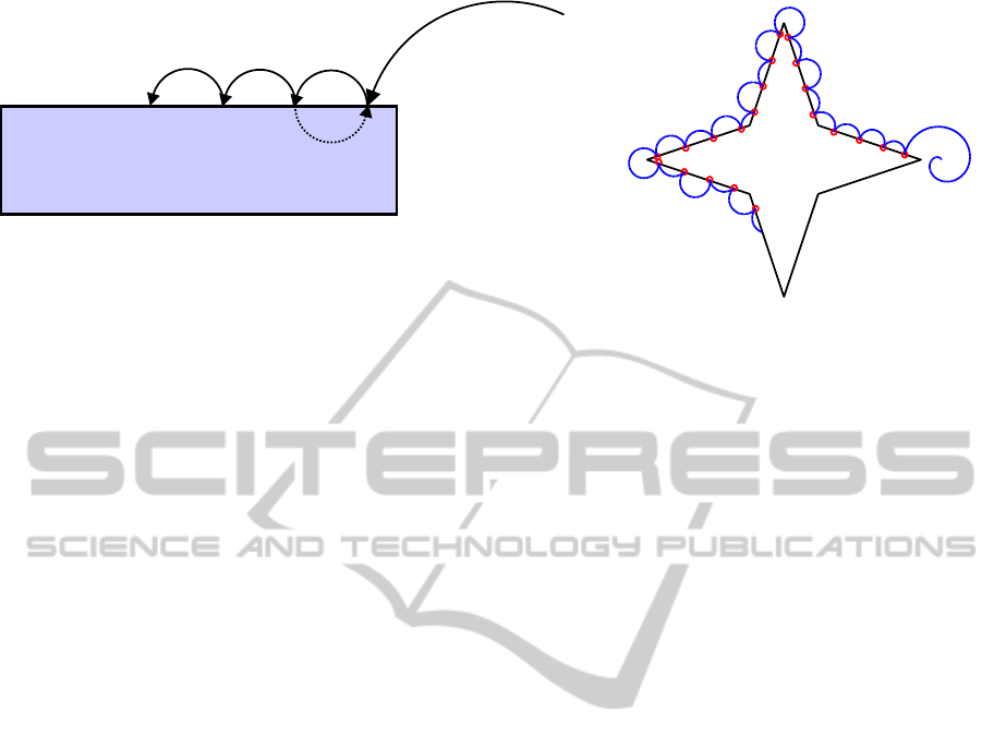
A B
Figure 2: A: Core idea of Contour-Net. Each contact induces a 180
◦
phase forwarding of a circular movement. Combined
with velocity control of a tactile probe, the resulting change in movement velocity and direction causes the probe to “bounce
off” the surface at every contact event, resulting in a successive scan along the object’s shape. B: 2D simulation of contact-
triggered contour tracing. Black: star-shaped object. Blue: trajectory of the antennal tip. Red dots: contact locations.
of the oscillator. Second, it is simple and well de-
fined in terms of amplitude, phase and frequency,
which can be adjusted independently from each other.
Because of these properties, smooth online modula-
tion of trajectories can be achieved through chang-
ing parameters of the system at run-time. More-
over, these properties help in entrainment of the CPG
rhythm through sensory feedback, e.g., when be-
ing coupled with a mechanical system (Righetti and
Ijspeert, 2006). Hopf CPG’s have been applied suc-
cessfully to biped (Buchli et al., 2005; Righetti and
Ijspeert, 2006) and quadruped (Brambilla et al., 2006;
Ijspeert et al., 2007) locomotion.
2.2 Contact-triggered Contour Tracing
The basic idea of the contour-tracing model, as illus-
trated in figure 2A, is that each contact event triggers
a phase shift in the cyclic sampling movement of the
antenna. Ideally, this phase shift should cause the an-
tenna to “bounce off” the object after each contact.
Using a Hopf Oscillator to control the antennal posi-
tion directly would require memorizing the location
of the centre of oscillation, and shifting it along the
object surface. The need for a memory structure can
be avoided if the Hopf Oscillator output is used to
set the antennal velocity rather than position. Figure
2B shows the “scan path” (in analogy to eye-tracking
scan paths) along a star-shaped 2D-object. The veloc-
ity commands applied to the antennal joints, α and β
are given by:
∆α = s
1
x
∆β = s
2
y
where s
1
and s
2
are scaling factors, setting the max-
imum action range of the antenna. Setting these fac-
tors to distinct values leads to ellipsoid trajectories as
found in stick insect antennal movements (Krause and
Dürr, 2004).
The 2D simulation shown in figure 2B
was implemented in Matlab and contact loca-
tions are calculated using the Geom2D toolbox
(http://matgeom.sourceforge.net).The simulated an-
tenna and the Hopf Oscillator equations are iterated
using first order, forward Euler Integration with a
fixed time step ∆t.
After a contact is detected by the antenna, the
amplitude µ and the frequency ω are immediately
switched from a large amplitude, low frequency
“searching mode” to a high-frequency, low ampli-
tude “sampling mode”. Once a certain time span
T
sampling
has passed without encountering a further
contact event, the parameters are switched back to the
“searching mode” pattern.
A 180
◦
phase shift can be easily implemented by
negating the Hopf Oscillator state variables: x
t+1
=
−x
t
and y
t+1
= −y
t
. Because of the discrete-time na-
ture of numerical simulations, contacts with an obsta-
cle may last longer than a single time step. Therefore,
the 180
◦
phase shift should be applied only once for
each contact event. In the block diagram in figure 1,
this is indicated by the discrete pulse block.
2.3 Robustness Evaluation
The robustness of the contour tracing algorithm was
evaluated by scanning a rough surface. For genera-
tion of a random contour, we tested shapes with lin-
ear segments of random orientation and length. The
goal for the algorithm was to completely scan the sur-
face from the right to the left outermost side with-
out getting stuck, see figure 3A for a sample surface.
The surface was structured as a 10 units long, initially
straight line with 40 uniform segments. The locations
(x
i
, y
i
) of the nodes connecting the segments were
ICAART2014-InternationalConferenceonAgentsandArtificialIntelligence
94
0 2 4 6 8 10
90
92
94
96
98
100
noise level
success rate [%]
A B
Figure 3: Robustness evaluation of the contour-tracing algorithm. A: Extreme example, in which the antenna got trapped in a
cavity of the random contour. B: Success rate of contour-tracing in percentage. N=100 trials.
Table 1: Simulation parameters.
parameters 2D-Sim 3D-Sim
γ 4.0 4.0
µ
searching
1.0 0.5
µ
sampling
0.2 0.1
ω
searching
1.0 1.0
ω
sampling
2.0 2.0
∆t 0.02 0.02
s
1
= s
2
1.0 0.5
then randomized by x
i
= x
i
+ 0.15 ∗ rand(−r, r) and
y
i
= y
i
+rand(−r, r) where rand(−r, r) generates uni-
formly distributed random numbers between −r and
r. N=100 trials were performed for each noise level
r = 0.5, 1, .., 10. In almost all trials, the rough surface
could be completely scanned from start to end. Fig-
ure 3A shows one of the rare cases, where the contour
tracing algorithm got trapped in a cavity. Figure 3B
shows the overall success rate, i.e. the percentage of
trials that completely scanned the rough surface.
2.4 3D Simulation
The contour tracing algorithm also works reliably in
3D space. Virtually no change in the algorithm is re-
quired, except minor parameter tuning, see table 1.
Figure 4 shows a kinematic antennal model with or-
thogonal joint axes (similar to a cardan joint), probing
several complex objects like a Torus or a Octahedron.
Contact events were calculated using the Geom3D
Matlab package, including the contact distance along
the tactile probe.
3 TACTILE SHAPE
RECOGNITION
An application scenario for Contour-Net is tactile
shape recognition of sampled objects. Each contact
point with the surface can deliver direct information
about the contact distance, the current joint angles at
contact time and indirect values like the state of the
Hopf Oscillator. Collecting these values should al-
low a discrimination of object shapes based on pre-
vious learned examples. Here, we apply a plain but
large feed-forward neural network to solve the classi-
fication task. Previous results have shown that mul-
tilayer neural networks can classify hand-written dig-
its and temporal eye-tracking data with minimal pre-
processing, only (Krause et al., 2013a). We propose to
feed the collected and normalised contact-point data
directly as input values to the network. Normalisation
rescales the different data components to a range from
[−1, 1].
Due to the well known curse of dimensionality
problem (shrinking norm, Beyer et al. (1999)), the
training dataset should be as large as possible, requir-
ing long training times with common neural network
training algorithms. For example, standard back-
propagation has to deal with local minima (LeCun
et al., 1998) and vanishing gradients (Hochreiter et al.,
2001). Using No-Prop-fast (Krause et al., 2013a), a
special case of an Extreme Learning Machine (Huang
et al., 2006), these problems can be circumvented
and almost interactive training times can be achieved.
This allows the generation of parameter tuning curves
with many repetitions of the learning process using
personal computers.
3.1 Training Dataset
To collect a large training dataset, four different 2D-
shapes (triangle, square, star, circle) were traced us-
ing Contour-Net. The shape size was scaled between
100% and 200%, shapes were rotated randomly be-
tween 0
◦
and 360
◦
, and the initial contact location was
also randomized. Figure 6 shows a small sample from
Contour-Net-AModelforTactileContour-tracingandShape-recognition
95
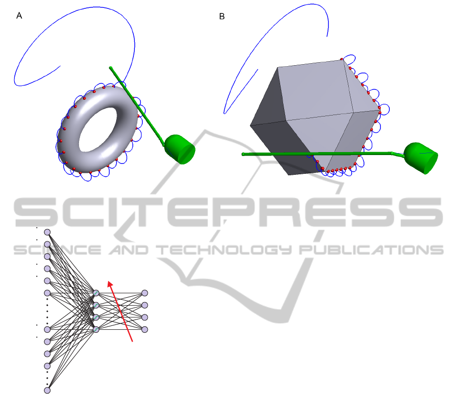
Figure 4: 3D simulation of contact triggered contour tracing. Grey: objects. Green: insect head with left antenna. Blue:
trajectory of the antennal tip. Red dots: contact locations. A: torus, B: octahedron.
x
1
y
1
d
1
x
2
y
2
d
2
x
n
y
n
d
n
0
bias=1
0 „triangle“
1 „square“
0 „circle“
linear output
layer
fixed
hidden layer
0 „star“
Figure 5: General network structure used for shape recog-
nition. A plain feed forward network with a large hidden
layer is used. Data components ( ˙x, ˙y from Hopf Oscilla-
tor, contact distance d along antenna) collected during a
contour-sampling are serialized, rescaled to the range -1 to
1 and fed into the network. Shorter contour-scans can be
zero-padded. Hidden layer weight values are initialized ran-
domly and only the output layer is trained (see text). Class
labels use a “one-out-of-n” coding.
the 2D-dataset. A fixed number of contact points was
selected such that all shapes in all sizes were ’encir-
cled’ at least once, hence completely traced. 400 ran-
dom samples with 35 contact points per shape were
collected, resulting in a training dataset with 1600
samples. Each contact point consisted of 3 compo-
nents: the ˙x and ˙y velocity components of the Hopf
Oscillator and the object size. Hence, the raw input to
the neural network has 105 dimensions. The network
has one hidden layer and 4 outputs. Output values use
a “one-out-of-n” coding scheme. The hidden layer
of No-Prop networks (Widrow et al., 2013) is fixed
and was initialized with uniformly distributed random
numbers. Figure 5 shows the general network struc-
ture.
3.2 Classification Performance
25 randomly initialized networks were trained on the
dataset, and performance was evaluated using 10-fold
cross validation. Figure 7B shows how the classifica-
tion accuracy depends on the hidden layer size. As
shown in Krause et al. (2013a), essentially two com-
ponents influence the performance: the hidden layer
size and the hidden layer weight range. The optimal
weight range of hidden layer units does not depend
on the number of hidden layer units (figure 8) but on
the number of inputs and was estimated to be from -
0.5 to 0.5 for both the 2D and 3D training dataset (see
section 3.3). Figure 7B (blue curve) shows that an
acceptable, size- and rotation-invariant shape classifi-
cation can be achieved. The discrimination rate peaks
around 600 hidden units and decreases after that. The
low spread of performance values indicates that the
algorithm has not to deal with local minima. This is
a favourable feature of the No-Prop method, see also
Widrow et al. (2013).
Yet, contour tracing trajectories were found to be
fairly variable, depending on angle of attack of the
tactile probe relative to the surface. Figure 7A shows
an example where the probe arrives at a flat angle to
the surface. The subsequent, contact-induced 180
◦
phase shift of the oscillator causes the probe to leave
the surface in a suboptimal, backward direction. The
resulting pattern alternates between a flat and large
arc.
ICAART2014-InternationalConferenceonAgentsandArtificialIntelligence
96
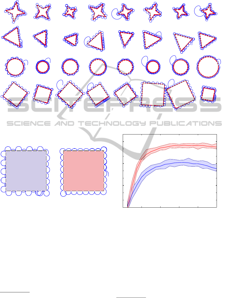
Figure 6: Sample collection of the four different shapes used for the classification task. The size and orientation of the shapes
as well as the initial contact location was randomized.
0 200 400 600 800 1000
50
55
60
65
70
75
80
85
90
95
100
hidden layer size
classification accuracy [%]
CBA
Figure 7: Classification results improve after incorporating surface-normal information into Contour-Net. A: Sampling trajec-
tory using a fixed 180
◦
phase shift of the Hopf Oscillator after contact. B: The phase of the oscillator is set such that the tactile
probe leaves the object surface in the normal direction after a contact. The resulting sampling trajectory is more regular. C:
Classification accuracy using a fixed phase shift (blue), and variable phase shift depending on the object surface normal (red).
A training dataset with four shapes as shown in figure 6 with n=400 samples per shape was used. N=25 repetitions. Solid
curve = mean value, shaded area = min and max values.
Approaching a surface perpendicular with an op-
timal, 90
◦
angle, not only avoids potential slip, see
Kaneko et al. (1995). Improving the regularity of the
scan path might also improve the shape classification
performance. A simple solution would be to use the
estimated surface normal
1
for setting the outgoing
1
In the simulation, the surface normal was estimated by
a local, 360
◦
subsampling of the surface around the contact
position. From the resulting list of intersections with the
angle after contact. Figure 7B shows an example of
an improved sampling trajectory. The main advan-
tage for the classificator is a lower spread of contact
parameters along flat regions of an object and a more
pronounced change in values at sharp edges. This is
reflected in more than 10% improvement of the classi-
fication accuracy. Figure 7C, red curve, shows the im-
object, an average surface normal vector could be calculated
similar to the mean resultant vector in circular statistics.
Contour-Net-AModelforTactileContour-tracingandShape-recognition
97
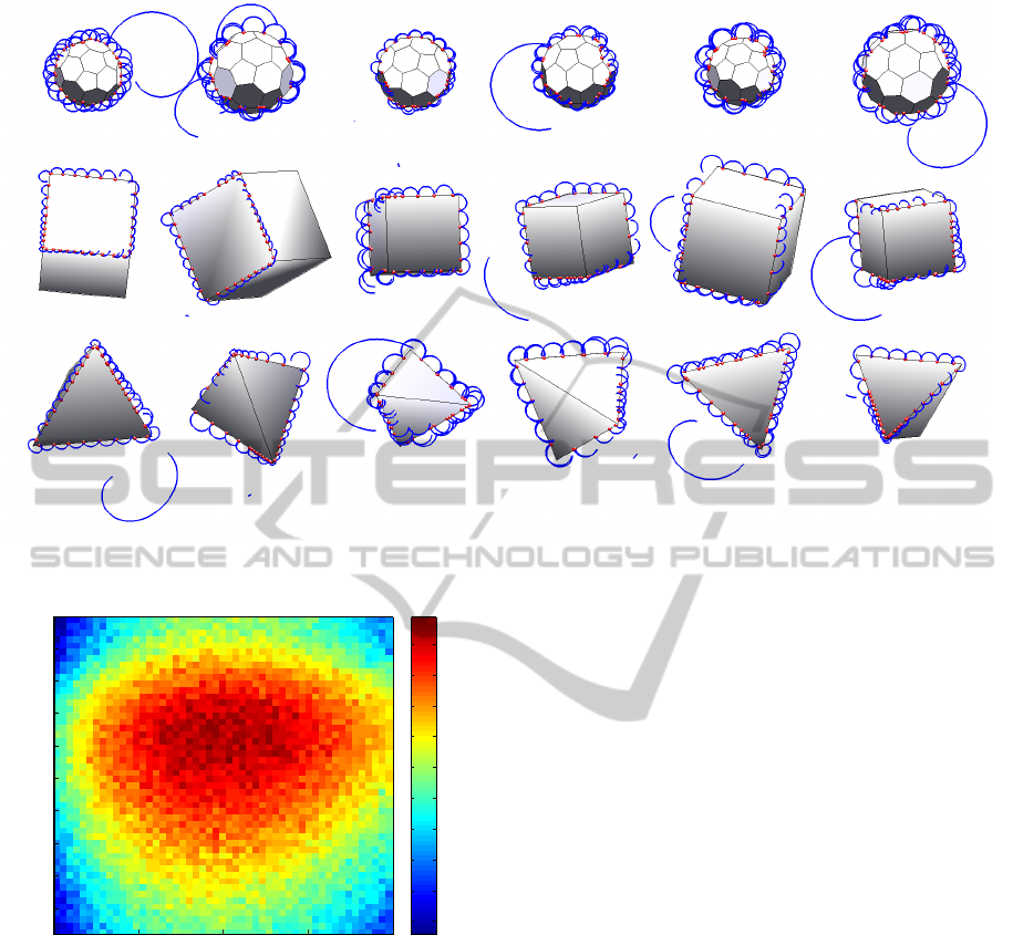
Figure 9: Sample collection of three different 3D objects: 1. row: soccer ball; 2. row: cube; 3. row: tetrahedron. The size,
position and spatial orientation of the shapes as well as the initial antennal location were randomized.
78.5
79
79.5
80
80.5
81
81.5
82
82.5
83
hidden layer size
500 15001000750 1250
weight range
0.1
0.2
0.3
0.4
0.5
0.6
0.7
0.8
0.9
1
Figure 8: Classification accuracy (color coded) depend-
ing on weight range and hidden layer size. Used training
dataset: 3D shapes, n=1000 samples per shape, n=20 repe-
titions. The optimal weight range value is independent from
the hidden layer size.
proved recognition rate using a dataset identical in pa-
rameters to section 3.2, but generated using Contour-
Net with variable phase shift depending on the surface
normal.
3.3 3D Shape Classification
Subsequently, classification performance using 3D
objects was tested. Three different objects were
used: a soccer ball, a cube and a tetrahedron, see
figure 9. The objects were scaled between 100%
and 150%; placed at a random position (x, y, z) =
[20..30, −5..5, −5..5] in front of the antenna; and ro-
tated randomly around all axes in the full range of
360
◦
. The initial antennal location around the object
was also randomized. Three datasets with 400, 1000
and 3000 random samples per shape with 35 contact
points per shape were collected. From each contact
event, three components were used: the ˙x and ˙y values
of the Hopf Oscillator and the contact distance along
the antenna. The neural network had 105 inputs and
three outputs.
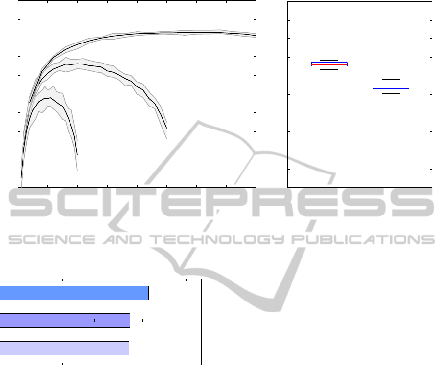
Figure 10 shows the classification accuracy for the
three differently sized datasets. The increased com-
plexity of the task required a very large dataset to
achieve a classification rate above 90%. Due to the
random rotation around all axes, the supervised learn-
ing algorithm has to be trained on a sufficiently large
number of contour projections of the objects. Re-
stricting the task to a fixed object size and to a random
rotation around a single axis, only, would certainly re-
duce the necessary size of the training dataset. Figure
10B shows that the contact distance information only
slightly improved classification performance by 5%.
Hence, the contact distance along the antenna is not
essential and does not need to be very precise or may
be omitted completely.
3.4 Performance Evaluation
The No-Prop-fast method was compared with two
ICAART2014-InternationalConferenceonAgentsandArtificialIntelligence
98
0 500 1000 1500 2000 2500 3000 3500 4000
50
55
60
65
70
75
80
85
90
95
100
hidden layer size
classification accuracy [%]
distance,
dx, dy
dx, dy
1200 samples
n = 25
3000 samples
n=25
n=25
3000 samples
n = 25
9000 samples
n = 10
A B
Figure 10: 3D shape classification performance strongly depends on the sample size. A: Performance for three different
sample sizes. The neural network requires a fairly large sample size to achieve high performance. It needs to “see” several
contour projections of the randomly oriented objects. B: Influence of the input components on performance. Performance is
still good with the velocity components of the Hopf Oscillator, only.
50 60 70 80 90 100
No-Prop-fast: 91.6%
backprop- : 91.9%scg
support vector machine - rbf: 98.0%
cpu time [s]
3D dataset, 9000 samples, n=25
3.0 ± 0.1
146.8 ± 0.7
19.8 ± 1.0
Figure 11: Classification accuracy and training times
of three different algorithms. First row: No-Prop-fast
(n
hidden
= 3000), second row: scaled conjugate gradients
backpropagation (n
hidden
= 64), third row: gaussian kernel
support vector machine. Bars show median, whiskers show
min and max values, CPU times are given as mean±SD.
other algorithms, the default pattern classification al-
gorithm of the Matlab 2012a neural network toolbox,
scaled conjugate gradient backpropagation (BP
scg
)
and an implementation of a gaussian kernel support
vector machine (SVM
rb f
) found in the Matlab 2012a
statistics toolbox. Figure 11 shows recognition rates
and CPU times of these algorithms, applied to the
3D shape dataset with 9000 patterns. CPU time mea-
surements were performed on a Dell Precision T3500
Workstation (Intel Xeon W3530 CPU at 2.8 GHz with
8 Mbyte second level cache) running Windows 7. The
three different algorithms were evaluated using ten-
fold cross-validation and 25 repetitions with random-
ized samples and randomly initialized networks.
A separate SVM
rb f
was trained for each shape
(one-against-all classification), using the matlab
function ’svmtrain’ with sigma_rb f = 4.2 and
boxconstraint = 10. All other parameters were kept
at their default values. The performance of BP
scg
was
tested using a feedforward network with a single hid-
den layer (64 units), created with the Matlab function
’patternnet’ and trained with all parameters at their
default values. SVM
rb f
achieved the highest median
recognition rate (98%). Recognition rates of BP
scg
were lower (92%) with high spread, but individual
networks achieved up to 96%. No-Prop-fast follows
with 91%.
While the recognition rates of all three algorithms
are above 90%, training times were found to differ
significantly. Values given in figure 11 show the aver-
age duration of individual training runs (n=250). The
Matlab implementation of SVM
rb f
required almost
147 seconds to learn the dataset, while No-Prop-fast
required only three seconds. Hence, for the shape
recognition task, No-Prop-fast is approximately 50
times faster than SVM
rb f
and still six times faster than
the Matlab implementation of one of the fastest BP-
algorithms.
4 CONCLUSIONS
Contour-Net is a robust, bio-inspired method for tac-
tile contour-tracing. In its simplest instantiation, it
Contour-Net-AModelforTactileContour-tracingandShape-recognition
99

requires only a single, binary signal: if the antenna
or tactile sensor is in contact with an object or not.
Yet, the model captures essential behaviours observed
in its natural paragon, the stick insect antenna (Dürr
et al., 2001). For example, it implements the contact-
induced switch from a large amplitude searching be-
haviour to a local, higher frequency sampling of an
object (Krause et al., 2013b). Contour-Net can be eas-
ily extended to use two or more antennae including
mutual coordination and attentive visual target track-
ing, as will be shown in a follow-up paper.
Raw, minimally pre-processed (normalisation)
data collected from contact events was sufficient to
achieve rotation-, size- and position- invariant shape
recognition rates of over 90% using a plain feed-
forward neural network. A drawback for robotic ap-
plications is that the training dataset needs to be fairly
large. Instead of using raw data as the network input,
extracting higher level features from collected con-
tour points should significantly reduce the required
amount of training samples. Possible features might
be the average Euclidean distance and the spread of
Hopf Oscillator phase differences between successive
contact points. An unsupervised learning algorithm
(SOM; Boltzmann Machine) will be closer to nat-
ural, continuous learning (automatic clustering with
delayed categorization).
We have further shown that incorporating surface
normal information will improve not only the regu-
larity of the sampling trajectory, but also improve the
recognition performance of a neural network. Hit-
ting a surface perpendicular can potentially reduce
slip of an insect antenna inspired robotic tactile sensor
(Kaneko et al., 1995). The reliable and fast detection
of the surface normal using a tactile sensor will be a
challenging and interesting task.
ACKNOWLEDGEMENTS
This work was supported by EU grant EMICAB
(FP7-ICT, grant no. 270182) to Prof. Volker Dürr.
We thank Prof. Holk Cruse for valuable comments on
earlier versions of the manuscript.
REFERENCES
Beyer, K., Goldstein, J., Ramakrishnan, R., and Shaft, U.
(1999). When is "nearest neighbor" meaningful? In
Beeri, C. and Buneman, P., editors, Database Theory -
ICDT 99, volume 1540 of Lecture Notes in Computer
Science, pages 217–235. Springer Berlin Heidelberg.
Brambilla, G., Buchli, J., and Ijspeert, A. (2006). Adap-
tive four legged locomotion control based on nonlin-
ear dynamical systems. In From Animals to Animats
9. Proceedings of the Nineth International Conference
on the Simulation of Adaptive Behavior (SAB 06).
Buchli, J., Righetti, L., and Ijspeert, A. J. (2005). A dy-
namical systems approach to learning: a frequency-
adaptive hopper robot. In Proceedings of the VIIIth
European Conference on Artificial Life (ECAL 2005),
Lecture Notes in Artificial Intelligence, pages 210–
212.
Dürr, V., König, Y., and Kittmann, R. (2001). The anten-
nal motor system of the stick insect Carausius mo-
rosus: Anatomy and antennal movement pattern dur-
ing walking. Journal of Comparative Physiology A,
187(2):131–144.
Erber, J., Kierzek, S., Sander, E., and Grandy, K. (1998).
Tactile learning in the honeybee. Journal of Compar-
ative Physiology A, 183:737–744.
Esslen, J. and Kaissling, K.-E. (1976). Zahl und
verteilung antennaler sensillen bei der honigbiene
(Apis mellifera l.). Zoomorphology, 83:227–251.
10.1007/BF00993511.
Hochreiter, S., Bengio, Y., Frasconi, P., and Schmidhuber, J.
(2001). Gradient flow in recurrent nets: the difficulty
of learning long-term dependencies. In S. C. Kremer,
J. F. K., editor, A Field Guide to Dynamical Recurrent
Neural Networks. IEEE Press.
Hoinville, T., Wehner, R., and Cruse, H. (2012). Learn-
ing and retrieval of memory elements in a navigation
task. In Prescott, T., Lepora, N., Mura, A., and Ver-
schure, P., editors, Biomimetic and Biohybrid Systems,
volume 7375 of Lecture Notes in Computer Science,
pages 120–131. Springer Berlin Heidelberg.
Huang, G.-B., Zhu, Q.-Y., and Siew, C.-K. (2006). Extreme
learning machine: Theory and applications. Neuro-
computing, 70(1-3):489 – 501.
Ijspeert, A. J. (2008). Central pattern generators for loco-
motion control in animals and robots: A review. Neu-
ral Networks, 21(4):642 – 653.
Ijspeert, A. J., Crespi, A., Ryczko, D., and Cabelguen, J.-
M. (2007). From swimming to walking with a sala-
mander robot driven by a spinal cord model. Science,
315(5817):1416–1420.
Kaneko, M., Kanayama, N., and Tsuji, T. (1995). 3-d active
antenna for contact sensing. In IEEE International
Conference on Robotics and Automation, volume 1,
pages 1113–1119. IEEE.
Kaneko, M., Kanayma, N., and Tsuji, T. (1998). Active
antenna for contact sensing. IEEE Transactions on
Robotics and Automation, 14(2):278–291.
Kevan, P. G. and Lane, M. A. (1985). Flower petal micro-
texture is a tactile cue for bees. Proceedings of the
National Academy of Sciences, 82(14):4750–4752.
Kim, D. and Möller, R. (2007). Biomimetic whiskers for
shape recognition. Robotics and Autonomous Systems,
55(3):229–243.
Krause, A. F. and Dürr, V. (2004). Tactile efficiency of in-
sect antennae with two hinge joints. Biological Cy-
bernetics, 91(3):168–181.
Krause, A. F. and Dürr, V. (2012). Active tactile sampling
ICAART2014-InternationalConferenceonAgentsandArtificialIntelligence
100

by an insect in a step-climbing paradigm. Frontiers in
Behavioural Neuroscience, 6(30):1–17.
Krause, A. F., Essig, K., Piefke, M., and Schack, T. (2013a).
No-prop-fast - a high-speed multilayer neural net-
work learning algorithm: Mnist benchmark and eye-
tracking data classification. In Engineering Applica-
tions of Neural Networks (EANN 2013), pages 446–
455. Springer.
Krause, A. F., Winkler, A., and Dürr, V. (2013b). Cen-
tral drive and proprioceptive control of antennal
movements in the walking stick insect. Journal of
Physiology-Paris, 107(1-2):116 – 129.
LeCun, Y., Bottou, L., Orr, G. B., and Müller, K.-R. (1998).
Efficient backprop. In Orr, G. B. and Müller, K.-R.,
editors, Neural Networks: Tricks of the Trade, volume
1524 of Lecture Notes in Computer Science, pages 9–
50. Springer Berlin Heidelberg.
Lederman, S. and Klatzky, R. (2009). Haptic perception:
A tutorial. Attention, Perception, & Psychophysics,
71(7):1439–1459. 10.3758/APP.71.7.1439.
Lee, M. and Nicholls, H. (1999). Review article tactile sens-
ing for mechatronics - a state of the art survey. Mecha-
tronics, 9(1):1 – 31.
Patanè, L., Hellbach, S., Krause, A. F., Arena, P., and Dürr,
V. (2012). An insect-inspired bionic sensor for tac-
tile localization and material classification with state-
dependent modulation. Frontiers in Neurorobotics,
6(8):1–18.
Righetti, L. and Ijspeert, A. J. (2006). Programmable cen-
tral pattern generators: an application to biped loco-
motion control. In IEEE International Conference on
Robotics and Automation (ICRA), pages 1585–1590.
IEEE.
Russell, R. A. and Wijaya, J. A. (2003). Object location and
recognition using whisker sensors. In Australasian
Conference on Robotics and Automation, pages 761–
768.
Schilling, M., Hoinville, T., Schmitz, J., and Cruse, H.
(2013). Walknet, a bio-inspired controller for hexapod
walking. Biological Cybernetics, 107(4):397–419.
Schütz, C. and Dürr, V. (2011). Active tactile exploration
for adaptive locomotion in the stick insect. Philosoph-
ical Transactions of the Royal Society B: Biological
Sciences, 366(1581):2996–3005.
Solomon, J. H. and Hartmann, M. J. (2006). Biomechan-
ics: Robotic whiskers used to sense features. Nature,
443(7111):525.
Staudacher, E., Gebhardt, M. J., and Dürr, V. (2005). Anten-
nal movements and mechanoreception: neurobiology
of active tactile sensors. Advances in Insect Physiol-
ogy, 32:49 – 205.
Widrow, B., Greenblatt, A., Kim, Y., and Park, D. (2013).
The No-Prop algorithm: A new learning algorithm
for multilayer neural networks. Neural Networks,
37:182–188.
Contour-Net-AModelforTactileContour-tracingandShape-recognition
101
