
Image Quality Assessment using ANFIS Approach
El-Sayed M. El-Alfy and Mohammed R. Riaz
College of Computer Scineces and Engineering, King Fahd University of Petroleum and Minerals,
Dharan 31261, Saudi Arabia
Keywords: Image Quality Assessment, Adaptive Neuro-fuzzy Inference System, ANFIS, Differential Mean Opinion
Score, Human Visual System, Subjective Assessment, Objective Assessment.
Abstract: Due to the increasing use of digital images in electronic systems, it becomes important to evaluate the
degradation in image quality during acquisition, processing, storage and transmission. In this paper, we
investigate the ability of the adaptive neuro-fuzzy inference system (ANFIS) for quality assessment of
digital images with respect to original (reference) images. Several metrics for objective quality assessment
are calculated and used as inputs to an adaptive fuzzy inference system which in turn estimates a differential
mean opinion score (DMOS) for different types of distortions. The predicted values are compared with the
actual DMOS values using correlation and error measures. With 7-input ANFIS network, the results show
that predicted DMOS values are highly correlated to the actual values using a publicly available and
subjectively rated image database. For example, for distorted images due to JPEG 2000 compression, the
attained results for correlation coefficient, Spearman’s ranked correlation, and RMSE are 0.9944, 0.9902,
and 3.32, respectively. These results show that combining the advantages of neural networks with fuzzy
systems can be a promising approach for predicting the subjective quality of digital images.
1 INTRODUCTION
Digital images are gaining great importance in the
domain of electronic technology in recent years.
However, images can be corrupted due to various
reasons during acquisition, processing, storage and
transmission. With the increasing use of digital
imaging systems such as digital cameras, high
definition cameras, monitors and printers, Image
Quality Assessment (IQA) has attracted great
attention in image processing applications (Kudelka
Jr., 2012). Moreover, a variety of image processing
techniques can benefit from image quality
assessment for adaptive parameter tuning and
prediction of required resources.
Image quality assessment methods can be
classified into two main categories: subjective and
objective. The subjective assessment is conducted
through the human visual perception. Subjective
quality assessment is the optimal solution when
human beings are the ultimate recipients of the
image processing applications (Yi et al., 2008). To
reduce subjectivity, a group of human evaluators are
asked to visually judge the quality of a target image
as it relates to its original (reference) image. Then, a
Mean Opinion Score (MOS) is assigned to the target
image. This score can be scaled to range from 0
(very low quality) to 1 (very high quality). It can
also be expressed as differential MOS (DMOS)
which represents the difference between the scores
assigned to the reference and target images,
respectively. If we assume the reference image has
perfect quality, i.e. its MOS will be 1, then the range
for DMOS assigned to the target image will be from
0 (very high quality) to 1 (very low quality). Notice
that it is the opposite of MOS.
The automation of subjective quality assessment
is difficult as it depends on modelling the human
visual perception. In contrast, objective quality
assessment uses numeric measures to quantify the
degree of quality degradation. Hence, it can be
automated to replace the way a human assesses the
quality of an image. The majority of objective
quality assessment methods are based on pixel
difference metrics due to their low computational
complexity (Bouzerdoum et al., 2004). However,
these methods can suffer from some limitations in
dealing with the wide spectrum of image distortion
types. Hence, a number of other quality metrics have
been proposed in the literature for various situations
by different researchers (He et al., 2013).
169
M. El-Alfy E. and R. Riaz M..
Image Quality Assessment using ANFIS Approach.
DOI: 10.5220/0004823901690177
In Proceedings of the 6th International Conference on Agents and Artificial Intelligence (ICAART-2014), pages 169-177
ISBN: 978-989-758-015-4
Copyright
c
2014 SCITEPRESS (Science and Technology Publications, Lda.)

Whether subjective or objective, image quality
assessment techniques can be classified as no-
reference, full-reference or reduced-reference. This
classification depends on the availability of
information from the original image besides the
target or query image. In a no-reference technique,
the assessor has only access to the query image;
hence it is also termed as blind assessment, e.g. (De
and Sil, 2009; Li et al., 2011). But when the original
image is also available, it is termed as full-reference;
e.g. (Larson and Chandler, 2010). In some
applications, only partial information about the
original image can be available besides the query
image and hence it is termed reduced-reference
(Rehman and Wang, 2012).
This paper therefore explores the ability of
adaptive neuro-fuzzy inference system (ANFIS)
approach in predicting the subjective quality of
images. This is implemented through estimating a
combined score using a set of image quality metrics.
The predicted value is compared to the actual
differential mean opinion score (DMOS). We
consider five types of distortion at different levels
including JPEG compression, JPEG 2000
compression, additive pink Gaussian noise (APGN),
additive white Gaussian noise (AWGN) and
Gaussian blurring. The performance is evaluated and
compared in terms of Pearson’s correlation
coefficient, Spearman’s rank order correlation
coefficient, mean absolute error (MAE), and root
mean square error (RMSE).
The rest of the paper is structured as follows.
Section 2 gives a brief background of the main
ANFIS characteristics and how it can be used for
function approximation and prediction. The related
work is reviewed in Section 3. Section 4 provides
more details on image quality assessment and
defines the quality metrics that are used in this work.
Section 5 describes the dataset and discusses the
experimental work. Finally, Section 6 concludes the
paper and highlights future work.
2 BACKGROUND
In the case of fuzzy logic based systems, the
mapping of prior human knowledge or experience
into the inference process using linguistic variables
is an advantage but a cumbersome task. No standard
procedure is found to provide an efficient way of
this transformation. Usually, a trial and error
approach determines the type, size and settings of
the input and output membership functions (MFs).
Effective tuning methods for the input and output
membership functions and the reduction of the rule
base to the least necessary rules have always been on
the list of issues to be explored.
Adaptive neuro-fuzzy inference system or
ANFIS is emerged to mitigate the above mentioned
issues by providing a learning capability to the fuzzy
system through its integration with a neural network
(Jang, 1993). Thus, ANFIS combines the advantages
of both the fuzzy inference system and the neural
network. ANFIS has been widely used to solve
several problems in different domains (Balamurugan
and Rajesh, 2007; Khuntia and Panda, 2011;
Meharrar et al., 2011; Meena et al., 2012).
Figure 1: A typical example of an ANFIS architecture and
reasoning.
The ANFIS system works in two distinct phases.
The first phase is a neural-network phase, where a
system classifies data and finds patterns. The other
phase develops a fuzzy expert system through
adaptive tuning of membership functions (Khuntia
and Panda, 2011). Figure 1 shows a typical example
of a Sugeno-type ANFIS system, with two rules, two
inputs X and Y, and one output F. Each input
variable is assumed to have two terms (e.g. small
and large). This system consists of five layers; where
the output from each node in every layer is
represented by O
. Here, denotes the layer number
while the symbol denotes the neuron number
within the layer. The purpose of the first layer is to
fuzzify the crisp input values using a set of linguistic
terms (e.g., small, medium, and large). Membership
premises
consequents
x y
A1
A2
B2
B1
w
1
w
2
f
1
=p
1
x+q
1
y+r
1
f
2
=p
2
x+q
2
y+r
2
f=
w
1
f
1
+w
2
f
2
w
1
+w
2
ICAART2014-InternationalConferenceonAgentsandArtificialIntelligence
170

functions of these linguistic terms determine the
output of this layer as given by:
,
(1)
where
and
represent the membership
functions that establish the degree to which the
given input values and satisfy the quantifiers
and
. A variety of membership functions exists
such as bell-shaped, trapezoidal, triangular,
Gaussian, and sigmoidal.
The firing strength for each rule quantifies the
extent that any input data belongs to that rule, and is
computed in the second layer as the multiplication of
all the incoming signals at each node as follows:
∗
(2)
The nodes in the third layer perform
normalization operation by calculating the ratio of
the i-th rule’s firing strength to the sum of all rule’s
firing strengths as follows:
(3)
In Sugeno-type ANFIS system, the consequent
part of each rule is expressed as a linear combination
of the inputs. The fourth layer has square-shaped
nodes with node functions given as:
(4)
Finally, the last layer node conducts summation
of all incoming signals to generate the output as
weighted sum:
∑
∑
(5)
The objective of a learning algorithm is to update
the consequent and premise parameters in order to
achieve the least error between the predicted and the
desired target output. A hybrid training algorithm is
normally applied to tune the parameters of an
ANFIS network. Such a learning technique is
composed of least square estimates and a gradient
descend (back-propagation) algorithm. The first
stage updates the consequent parameters through
least-square estimates by passing of function signals
forward until layer 4. In the second stage, the error
rates are propagated backward which help in
updating the premise parameters by a gradient
descent algorithm.
3 RELATED WORK
In (Bouzerdoum et al., 2004), the authors proposed a
neural network approach for the assessment of
image quality. The neural network measured the
quality of an image by predicting the mean opinion
score (MOS) with the help of six key features
extracted from both the reference and target images.
These features are the two means, two standard
deviations, covariance and mean-square error. The
experimental work was carried out using 352 images
compressed by JPEG/JPEG2000. The resulting
correlation is about 0.9744 between the predicted
and actual MOS values. Similar work has been
conducted in (Kaya et al., 2011) where a neural
network approach is used to predict the subjective
image quality score DMOS using statisitical features
extracted from both the reference and target images.
In 2011, Li et al. developed a no-reference image
quality assessment using regression neural networks
to approximate the functional relationship between a
range of distortion types and the human subjective
judgment.
In (Yi et al., 2008), the authors developed an
image quality assessment method based on structural
distortion and image definition. They carried out
their experiments on ‘Lena’ and ‘Barbara’ original
and distorted images. In their work, it was shown
that the proposed method is more consistent with
human perception. In (Kung et al., 2010), the
authors used characteristics of structural similarity
index and artificial neural network for image quality
assessment. The experimental results showed that
their proposed approach can achieve adaptability for
image quality of different types. In (Lin and Kuo,
2011), the authors conducted a survey on perceptual
visual quality metrics, in which they compared the
commonly used 6 image metrics using seven public
image databases. In (Wee, 2010), a new full-
reference quality assessment metric is proposed to
automate the quality assessment of an image in the
discrete orthogonal moment domain. The metric was
constructed by using the spatial information of an
image using low-order moments.
When concerned with the use of ANFIS
approach in recent literature, in (Balamurugan and
Rajesh, 2007) the authors worked on classifying
greenery and non-greenery image classification
using ANFIS technique. They used a hybrid set of
parameters which involved texture and color
coherence vector (CCV). More recently in (Meena et
al., 2012), ANFIS was used for classification and
detection purposes for the brain Magnetic
Resonance (MR) images and tumor detection. The
decision making was performed in two stages. The
first stage involved using feature extraction using
principal component analysis (PCA) and in the
ImageQualityAssessmentusingANFISApproach
171

second stage, ANFIS was trained. The authors
mentioned that ANFIS, as a fuzzy logic based
paradigm, grasps the learning abilities of neural
network to improve the performance of the
intelligent system using a priori knowledge. The
authors demonstrated that ANFIS can be a
promising approach for image classification in the
field of medical sciences.
In (De and Sil, 2009), ANFIS is used to assess
quality of distorted/decompressed images without
reference to the original image using three statistical
features as inputs expressed as linguistic variables,
namely area, extent and eccentricity.
4 IMAGE QUALITY
ASSESSMENT
In this paper, we have developed a full-reference
quality assessment. The outline of the proposed
predictive model is shown in Figure 2. As a full-
reference method, the quality of a query image is
compared with a reference image of perfect quality.
Image quality is determined through various image
quality metrics computed based on features
extracted from the reference and target images.
These features are based on existing studies (Lin and
Kuo, 2011; Chetouani et al., 2010).
Here, we considered seven significant full-
reference quality metrics as follows:
Peak signal to noise ratio (PSNR)
Universal quality index (UQI)
Mean Structural similarity index (MSSIM)
Weighted Signal to Noise Ratio (WSNR)
Visual Information Fidelity (VIF)
Noise Quality Measure (NQM)
Information Fidelity Criterion(IFC)
These quality assessment measures are discussed
briefly in the following subsections.
4.1 Peak Signal-to-Noise Ratio (PSNR)
The traditional and most widely used objective
image quality assessment metric for many years is
the peak signal to noise ratio (PSNR). PSNR is a
pixel-based method, which means that the distorted
image and reference image are compared pixel by
pixel. The PSNR metric is a good measure for its
simplicity and power to assess white noise
distortion. However, a disadvantage of using it is
that it is inconsistent to human’s subjective
perception (Wang and Bovik, 2009). Moreover, it
may not capture the wide spectrum of distortion
Figure 2: Outline of the proposed ANFIS-based quality
assessment system.
types.
The peak signal to noise ratio between a
reference image and target image can be computed
utilizing the mean square error (MSE). For a
reference image A and target image B of size NM,
the mean square error is computed using:
1
(6)
where a
ij
and b
ij
are the gray levels of the pixels at
location (i, j) in the original and test images,
respectively. If we assumed 8-bit encoding for each
pixel, i.e. a maximum gray level of 255, then the
PSNR can be determined as follows:
10∗
255
(7)
4.2 Universal Quality Index (UQI)
Wang et al. (2004) proposed a universal quality
index (UQI) between target and reference images by
utilizing three different factors. The three factors are
luminance, contrast, and structural comparisons. The
luminance comparison , between a reference
image and a target image is determined in
terms of mean values
and
by the relation:
,
2
(8)
The contrast comparison
,
is performed
utilizing the standard deviations for images and
as:
,
2
(9)
Preprocessing
Compute
Quality
Metrics
ANFIS-
Based
Predictive
Model
Preprocessing
Predicted
DMOS
ICAART2014-InternationalConferenceonAgentsandArtificialIntelligence
172

Utilizing covariance between the images and,
the structural comparison
,
is given by:
,
2
(10)
Hence, the universal quality index is defined as:
,
,
,
,
4
(11)
The value of UQI lies between [-1, 1]. UQI is an
improved metric when compared to the PSNR.
4.3 Mean Structural Similarity Index
(MSSIM)
The structural similarity index (SSIM) measures the
similarity between two images (Wang et al., 2004).
This metric is an improved version of the UQI
resulting in improvement in the correlation between
the subjective and objective measures. The value of
SSIM lies between [0, 1] and is calculated as:
,
2
2
(12)
where
,
, L denotes the
dynamic range of pixel values, and K
1
and K
2
are
small positive constants. The SSIM index is
calculated for the whole image as one block.
However, when the features are highly spatially non-
stationary, SSIM can be calculated within local
windows and the overall image quality is measured
by the mean SSIM index as given by:
1
,
(13)
where K is the total number of local SSIM indices.
4.4 Weighted Signal-to-Noise Ratio
(WSNR)
In (Damera-Venkata et al., 2000), a different
approach to signal-to-noise ratio was used. It is
known as weighted signal-to-noise ratio (WSNR).
This measure is defined as the ratio of average
weighted signal power to the average weighted noise
power. Here, the contrast sensitivity functions (CSF)
are used as weights.
4.5 Visual Information Fidelity (VIF)
VIF metric was proposed by (Sheikh and Bovik,
2006). In this metric the image quality assessment
depends upon the amount of information shared
between the source (reference) image and the
distorted image. A fundamental limit is imposed on
how much information can flow from the source
image through the channel (i.e., the image distortion
process) to the receiver (i.e., human being). VIF is
distinctive over traditional image quality assessment
methods.
4.6 Noise Quality Measure (NQM)
NQM metric was proposed by (Damera-Venkata et
al., 2000) as a better measure for visual quality than
PSNR. It considers variation in contrast sensitivity
with distance, image dimensions and spatial
frequency. It also considers the variation in local
luminance, mean and contrast interaction between
spatial frequencies, and masking effects. NQM is
given by:
NQM (dB)=10 log
10
∑∑
∑∑
(14)
where a
ij
and b
ij
denote the (i,j) pixels in the
reference and distorted images.
4.7 Information Fidelity Criterion
(IFC)
IFC image quality assessment was proposed by
(Sheikh et al., 2005). This metric is based on natural
scene statistics. The IFC is the mutual information
between the source and distorted images. Firstly, the
mutual information is derived for one sub-band and
then generalized for multiple sub-bands. The IFC
quantifies the perceptual quality of the image.
5 EXPERIMENTS AND RESULTS
The images used in our study are collected from the
Oklahoma state university image database (also
known as CSIQ image database) (Larson and
Chandler, 2010). This image database is chosen for
our experiments because it has a large number of
images distorted with a variety of types. In addition,
it was previously used in several image quality
assessments in the literature, e.g. (Larson and
Chandler, 2010) and (Zhang et al., 2011).
The adopted dataset has 30 original images and
750 distorted versions of the original images. We
chose 5 types of distortions each is taken at five
levels (This means there are 530=150 images for
each distortion type). These distortions include
JPEG compression, JPEG 2000 compression,
additive pink Gaussian noise (APGN), additive
ImageQualityAssessmentusingANFISApproach
173
white Gaussian noise (AWGN) and Gaussian
blurring. Each image in the database is of 512512
pixels and each color has 256 levels (from 0 to 255).
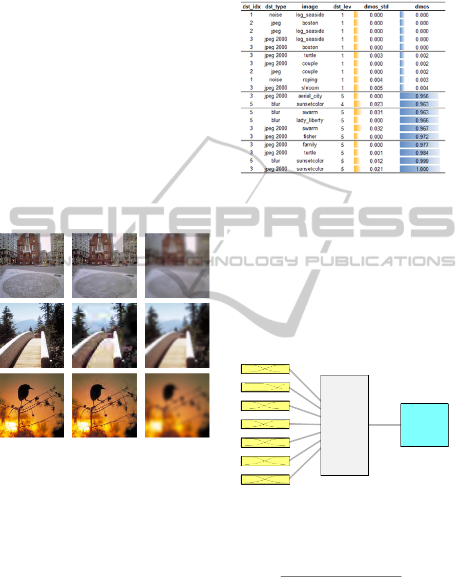
Examples of the images in this database are shown
in Figure 3.
Each distorted image in the database has a
subjective rating in the form of DMOS (Differential
Mean Opinion Score) ranging from 0 (no distortion
or lightly distorted) to 1 (highly distorted). Ratings
are conducted by 35 male and female observers with
ages from 21 to 35 years. The actual DMOS score
for each image pair is also taken from the Oklahoma
State University CSIQ image database website.
Figure 4 shows distorted images with top ten and
bottom ten DMOS ratings including distortion name
and index, image name, distortion level, standard
deviation of DMOS, and DMOS. It is clear that
rating is high when the level of distortion is high and
vice versa.
(a) Original b) JPEG 2000 c) Blur
Figure 3: Examples of the images in CSIQ database for
two types of distortions JPEG 2000 and Gaussian Blur.
We paired each distorted image with the
corresponding original image as a reference. This
gave us 750 pairs. Out of the 750 image pairs, we
used 600 pairs for training the model, 50 pairs for
validating the model and 100 pairs for testing the
model. Using MATLAB, we computed the seven
image quality measures under consideration (see
Section 4) using the code developed by their
inventors.
We then built different ANFIS models using
subsets of these measures and evaluated their
performances. The desired output of the ANFIS
Figure 4: Distorted images with top ten and bottom ten
DMOS ratings.
network was the crisp DMOS values. The first
ANFIS model has only three inputs (PSNR, UQI and
MSSIM) whereas the second ANFIS model has five
inputs (PSNR, UQI, MSSIM, WSNR and VIF). The
last ANFIS model has seven inputs (PSNR, UQI,
MSSIM, WSNR, VIF, NQM, and IFC). Table 1
shows the ANFIS parameters and their values used
for training with 7 input variables. Figure 5 shows a
snapshot of the corresponding ANFIS model for the
7 input variables. The other two models use similar
parameter types but the values for input and output
MFs differs accordingly.
Figure 5: ANFIS model with 7 inputs.
For the purpose of evaluating the performance of
each model, we used four measures. The Pearson’s
linear correlation coefficient
is given by:
,
(15)
where
and
are vectors containing
the actual and predicted values for DMOS. To assess
the monotonicity relationship between predicted
value and actual value for a particular model, we
input1 (2)
input2 (2)
input3 (2)
input4 (2)
input5 (2)
input6 (2)
input7 (2)
f(u)
output (128)
(sugeno)
128 rules
ICAART2014-InternationalConferenceonAgentsandArtificialIntelligence
174

Table 1: ANFIS parameters and their values that are used
for training with 7 input variables.
ANFIS Parameter Value
N
umber of training data records 600
N
umber of validation data records 50
N
umber of testing
d
ata records 100
AND method Product
OR method
Probabilistic OR
(probor)
Implication method Product
Defuzzification method
Weighted average
(wtaver)
Aggregation method Sum
Output MF function Linear
Input MFs type
Generalized bell MF
(gbellmf)
N
umbe
r
of inputs 7
N
umber of outputs 1
N
umber of MFs per variable 2
N
umber of rules 128
used Spearman’s rank order coefficient
s.
This
measure is computed suing the same equation for
Pearson’s coefficient but replacing the raw scores by
their ranks. In order to find the error of the model,
we used Mean Absolute Error (MAE) and Root
Mean Square Error (RMSE) which as calculated as
follows:
1
|
|
(16)
1
(17)
where
and
are the actual and
predicted values for DMOS for the i-th image.
We started with the three features metrics PSNR,
UQI and MSSIM, selected arbitrarily as inputs to the
ANFIS network. The results of our experiment are
given in Table 2. In order to study the performance
as more features become available, we added two
more feature metrics, i.e. WSNR and VIF, and
repeated the experiment with a 5-input ANFIS
network. The corresponding results are shown in
Table 3. We again added two more feature metrics,
i.e. NQM and IFC, and repeated the experiment with
a 7-input ANFIS network and the yielded results are
shown in Table 4. The rationale behind repeating the
experiments was to judge the performance of the
ANFIS network by increasing the feature metrics
incrementally and document the results.
Considering the results in Tables 1, 2 and 3, we
can see that the predicted DMOS values are highly
correlated with the actual DMOS values for all
distortion types except APGN. The correlation
improves as more inputs become available. Similar
conclusions can be made regarding MAE and
RMSE.
For the sake of comparison, Figure 6 shows the
average values for the correlation of two types of
distortion JPEG/JPEG 2000 for our method and two
other methods from the literature: neural network
(Bouzerdoum et al., 2004) and MSSIM (Wang et al.,
2004). We should mention that the authors for the
other works used a different image database and
provided the results for only these two types of
distortions.
Table 2: Results for a 3-input ANFIS model (using PSNR,
UQI and MSSIM).
Distortion
s
MAE RMSE
Blur 0.9641 0.9665 5.4136 7.8199
JPEG 2000 0.9887 0.9837 3.9443 4.9776
JPEG 0.9477 0.9519 7.7900 10.3173
APGN 0.2413 0.6019 25.7500 60.2763
AWGN 0.9510 0.9562 11.4998 15.3729
Table 3: Results for a 5-input ANFIS model (using PSNR,
UQI, MSSIM, WSNR and VIF).
Distortion
s
MAE RMSE
Blur 0.9862 0.9811 3.3941 4.8836
JPEG 2000 0.9938 0.9881 2.6951 3.5981
JPEG 0.9762 0.9693 6.1521 7.8826
APGN 0.6181 0.7143 94.3118 98.5724
AWGN 0.9646 0.9636 16.7365 22.4688
ImageQualityAssessmentusingANFISApproach
175

Table 4: Results for a 7-input ANFIS model (using PSNR,
UQI, MSSIM, WSNR, VIF, NQM, and IFC).
Distortion
s
MAE RMSE
Blur 0.9937 0.9902 2.2626 3.2177
JPEG 2000 0.9944 0.9902 2.4395 3.3292
JPEG 0.9814 0.9758 5.7428 7.1629
APGN 0.7035 0.7338 96.1683 99.8975
AWGN 0.9548 0.9590 16.8990 22.7204
Figure 6: Comparing the average correlation results for
JPEG/JPEG 2000 distortion for three methods: ANFIS
with 7 inputs (proposed), neural network (NN)
(Bouzerdoum et al., 2004) and MSSIM (Wang et al.,
2004).
6 CONCLUSIONS
In this paper, we explored the application of an
adaptive neuro-fuzzy inference system (ANFIS) for
full-reference assessing the quality of images with
references. The experimental results showed that
ANFIS network can be trained using image quality
assessment metrics to predict the differential mean
opinion score (DMOS) with high correlation
coefficients and low errors. The ANFIS results
compare favourably with two other methods in the
literature. As a future work, the proposed method
can be evaluated using k-fold cross validation and
other databases. More quality assessment metrics
can be considered and in this case the selection of
the most relevant features for building the predictive
models will be of interest.
ACKNOWLEDGEMENTS
The authors would like to acknowledge the support
provided by the Deanship of Scientific Research at
King Fahd University of Petroleum & Minerals
(KFUPM). The authors would also like to thank the
anonymous reviewers for providing helpful and
constructive comments that helped enhancing the
paper presentation and content.
REFERENCES
Balamurugan, P., Rajesh, R., 2007. Greenery image and
non-greenery image classification using adaptive
neuro-fuzzy inference system. In International
Conference on Computational Intelligence and
Multimedia Applications.
Bouzerdoum, A., Havstad, A., Beghdadi. A., 2004. Image
quality assessment using a neural network approach.
In Fourth IEEE International Symposium on Signal
Processing and Information Technology.
Chetouani, A., Beghdadi, A., Deriche, M., 2010. Image
distortion analysis and classification scheme using a
neural approach. In 2nd European Workshop on
Visual Information Processing (EUVIP).
Damera-Venkata, N., Kite, T., Geisler, W., Evans, B.,
Bovik, A., 2000. Image quality assessment based on a
degradation model. IEEE Transactions on Image
Processing, 9(4): 636-650.
De, I., Sil, J., 2009. No-reference quality prediction of
distorted/decompressed images using ANFIS. In
International Conference on Computer Technology
and Development.
He, L., Gao, F., Hou W., Hao, L., 2013. Objective image
quality assessment: a survey. International Journal of
Computer Mathematics.
Kaya, S., Milanova, M., Talburt, J., Tsou, B., Altynova,
M. 2011. Subjective image quality prediction based
on neural network. In Proceedings of the 16th
International Conference on Information Quality.
Kudelka Jr., M., 2012. Image quality assessment. WDS'12
Proceedings of Contributed Papers, Part I, 94–99.
Kung, C.-H., Yang, W.-S., Huang, C.-Y., Kung, C.-M.,
2010. Investigation of the image quality assessment
using neural networks and structure similarity. In
Proceedings of the 3rd International Symposium
Computer Science and Computational Technology.
Jang, J. S. R., 1993. ANFIS: Adaptive-network-based
fuzzy inference system. IEEE Transactions on
Systems, Man, Cybernetics, 23(5/6):665–685.
Khuntia, S. R., Panda, S. 2011. ANFIS approach for SSSC
controller design for the improvement of transient
stability performance. Mathematical and Computer
Modelling, 57(1–2): 289–300.
Larson, E. C., Chandler, D. M. 2010. Most apparent
distortion: full-reference image quality assessment and
MSSIM NN ANFIS
Pearson
0,9114 0,9744 0,9879
Spearman
0,9499 0,969 0,983
0,86
0,88
0,9
0,92
0,94
0,96
0,98
1
ICAART2014-InternationalConferenceonAgentsandArtificialIntelligence
176

the role of strategy. Journal of Electronic Imaging, 19
(1): 011006: 1–011006:21.
Li, C., Bovik, A. C., Wu, X., 2011. Blind image quality
assessment using a general regression neural network.
IEEE Trans. Neural Network, 22(5): 793-799.
Lin, W., and Kuo, C-C., 2011. Perceptual visual quality
metrics: A survey. Journal of Visual Communication
and Image Representation, 22(4): 297–312.
Meena, R. S., Revathi, P., Begum, H. M. R., Singh, A. B.,
2012. Performance analysis of neural network and
ANFIS in brain MR image classification. In: S.
Patnaik & Y.-M. Yang (Eds.): Soft Computing
Techniques in Vision Sci., SCI 395, pp. 101–113.
Meharrar, A., Tioursi, M., Hatti, M., Stambouli, A., 2011.
A variable speed wind generator maximum power
tracking based on adaptive neuro-fuzzy inference
system. Expert Systems with Applications, 38(6):
7659–7664.
Rehman, A., Wang, Z., 2012. Reduced-reference image
quality assessment by structural similarity estimation.
IEEE Transactions on Image Processing, 21(8): 3378–
3389.
Sheikh, H.R., Bovik, A., De Veciana, G., 2005. An
information fidelity criterion for image quality
assessment using natural scene statistics. IEEE
Transactions on Image Processing, 14(12): 2117–
2128.
Sheikh, H. R., Bovik, A., 2006. Image information and
visual quality. IEEE Transactions on Image
Processing, 15(2): 430–444.
Wang, Z., Bovik, A. C., Sheikh, H. R., Simoncelli, E. P.,
2004. Image quality assessment: From error visibility
to structural similarity. IEEE Transactions on Image
Processing, 13(4): 600–612.
Wang, Z., Bovik, A. C., 2009. Mean squared error: Love it
or leave it? A new look at signal fidelity measures.
IEEE Signal Processing Magazine, 26(1):98–117.
Wee, C.-Y., Paramesran, R., Mukundan, R., Jiang, X.,
2010. Image quality assessment by discrete orthogonal
moments. Pattern Recognition 43(12): 4055–4068.
Yi, Y., Yu, X., Wang, L., Yang, Z., 2008. Image quality
assessment based on structural distortion and image
definition. International Conference on Computer
Science and Software Engineering.
Zhang, F., Ma, L., Li, S., Ngan, K. N., 2011. Practical
image quality metric applied to image coding. IEEE
Transactions on Multimedia, 13(4): 615–624.
ImageQualityAssessmentusingANFISApproach
177
