Region Segregation by Linking Keypoints Tuned to Colour
M. Farrajota, J. M. F. Rodrigues and J. M. H. du Buf
Vision Laboratory, LARSyS, University of the Algarve, 8005-139 Faro, Portugal
Keywords:
Colour, Segmentation, Keypoint, Cluster, Multi-scale, Visual Cortex.
Abstract:
Coloured regions can be segregated from each other by using colour-opponent mechanisms, colour contrast,
saturation and luminance. Here we address segmentation by using end-stopped cells tuned to colour instead
of to colour contrast. Colour information is coded in separate channels. By using multi-scale cortical end-
stopped cells tuned to colour, keypoint information in all channels is coded and mapped by multi-scale peaks.
Unsupervised segmentation is achieved by analysing the branches of these peaks, which yields the best-fitting
image regions.
1 INTRODUCTION
Motion, colour and form are inseparably intertwined
properties of objects in visual perception and in the
visual cortex (Hubel, 1995). Perceptual and psy-
chophysical studies have determined reciprocal links
between colour and form in human vision, and colour
has been found to impact the perception of form
(Shapley and Hawken, 2011). Also, perceptual
grouping plays a decisive role in visual perception
(Grossberg et al., 1997).
The capacity for colour vision requires multi-
ple sensors with different spectral absorption prop-
erties in combination with a nervous system which
is able to contrast signals (Jacobs, 2009). Trichro-
matic colour vision begins when the three types of
cones (photoreceptors with unique absorption spec-
tra) sample the irradiance across the retina (Derring-
ton et al., 2002). After retinal preprocessing, gan-
glion cells transmit the information from the eye to
the brain via the LGN (Gegenfurtner, 2003). In the vi-
sual cortex, single- and double-opponent V1 neurons
are part of an organisation that extends from V1 all the
way up to the inferotemporal cortex. Single-opponent
and double-opponent cells have different functions:
single-opponent cells respond to large coloured ar-
eas and inside those regions. Double-opponent cells
respond to coloured patterns, textures and colour
boundaries. Full colour segmentation in the brain is
supposed to occur in higher visual areas such as hV4
(Goddard et al., 2011; Roe et al., 2012), although
colour segmentation already begins in the early visual
areas V1 and V2 (Gegenfurtner, 2003).
Image segmentation and grouping are still big
challenges in computer vision. Many vision problems
can be solved by employing segmented images. That
is, when segmentations can be reliably and efficiently
computed. The use of more powerful computers has
led to a wide variety of segmentation methods (Pal
and Pal, 1993). A universal method does not yet exist.
Most techniques and variations are tailored to particu-
lar applications and they may work only under certain
conditions. For detailed surveys of colour segmenta-
tion see (Lucchese and Mitra, 2001; Mushrif and Ray,
2008; Vantaram and Saber, 2012).
In this paper we present a new colour segmenta-
tion model. Although this model does not employ any
prior information of the visual scene, it performs well
in most real-world scenarios and it works in real time.
We focus on colour information and spatial contrast
mechanisms to segment meaningful regions in a uni-
form colour space: CIE L*C*H. By applying multi-
scale cortical end-stopped cells tuned to colour, seg-
mentation can be achieved in an unsupervised way
and with a high degree of parallelism, yet robust to
noise and lighting conditions.
2 COLOUR SPACE AND COLOUR
CELLS
In increasingly higher visual areas of the cortex, cells
responsive to colour are increasingly more tuned to
specific and narrower ranges of hues (Gegenfurtner,
2003). This means that a wider range of cells can code
complex images into more regions with less percep-
247
Farrajota M., M. F. Rodrigues J. and M. H. du Buf J..
Region Segregation by Linking Keypoints Tuned to Colour.
DOI: 10.5220/0004827002470254
In Proceedings of the 3rd International Conference on Pattern Recognition Applications and Methods (ICPRAM-2014), pages 247-254
ISBN: 978-989-758-018-5
Copyright
c
 2014 SCITEPRESS (Science and Technology Publications, Lda.)

tual difference between similar colours. Our method
is not based on colour opponency or colour contrast
but on the colours themselves. In order to obtain
channels tuned to either colours or shades, we apply a
colour gain function in conjunction with a high-pass
function to the hue channels, and a low-pass function
to the chroma (saturation) channel. For applications
of region segmentation, a wider range of colours gen-
erally means more computations, hence a trade-off
between precision and speed is often required.
Here we use the CIE L*C*H* colour space. Let
image I(x,y) of size N × M be defined as (L
∗
,C
∗
,H
∗
):
luminance, chroma and hue. Figure 1 (bottom left) il-
lustrates hue H
∗
(x,y). We divide the hue circle into
N
ϕ
= 8 equal ranges (channels): φ
j
= j × 360/N
ϕ
and j = {1,2,...,N
ϕ
}. Each hue H
∗
(x,y) in each
channel φ
j
is weighted by a Gaussian gain func-
tion: G
φ
j
(x,y) = exp(−(H
∗
(x,y) − φ
j
)
2
/(2σ
2
)), with
σ = 360/N
ϕ
. In the next step, high-saturation hues
and low chromas are boosted in order to obtain eight
channels which code clear colours, and one chan-
nel which codes low saturation, i.e., shades. To
this purpose we apply two nonlinearities as defined
by the “low-pass” Butterworth function, BW (x,y) =
p
1/(1 +C
∗
(x,y)/K)
2η
, where C
∗
is chroma. The
“high-pass” function (1 − BW ) is applied to hues.
The high-pass BW function is applied to G
φ
j
,
which yields the colour responses Ψ
CC
j
(x,y) =
G
φ
j
(x,y) × (1 − BW (x,y)), with CC
j
= {1,..,N
ϕ
},
η = 3 and K = 6. As mentioned, the low-pass func-
tion is applied to chroma C
∗
to code low saturations:
Ψ
SC
(x,y) = BW (x,y) with K = 8. Finally, luminance
is not processed: Ψ
L
= L
∗
(x,y). Summarising, we
model 10 channels or 10 cells at each pixel position:
8 cells with boosted colours, one with low chroma
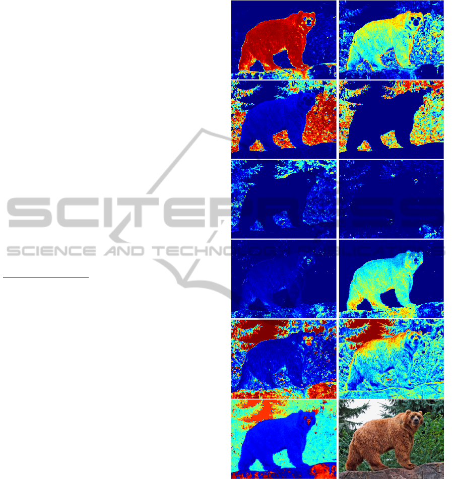
for shades, and one with luminance. Figure 1 shows
Ψ
CC
j
, Ψ
SC
and Ψ
L
. All responses Ψ are normalised
between 0 and 1 in each of the 10 maps.
3 MULTI-SCALE KEYPOINT
CELLS
Keypoints are based on cortical end-stopped cells
(Rodrigues and du Buf, 2006). The general idea be-
hind our region segmentation method is to perform
region fitting. One good way to achieve this is by
using Difference-of-Gaussian (DoG) filters, mainly
due to the desirable property of increasing visibility
of edges and other details around the borders of re-
gions (Young et al., 2001). Since end-stopped cells
employ derivatives, DoG filters can be approximated,
with additional benefits: (a) the particular orientation
Figure 1: Top four rows: colour responses Ψ
CC
j
, φ
j
=
{45
◦
,..., 360
◦
}. Fifth row: low saturation Ψ
SC
(left) and
luminance Ψ
L
(right). Bottom: hue H
∗
(left) and input im-
age.
of a region can be acquired, and (b) elongated, curved
and hollow (annulus) regions can be detected without
special solutions, i.e., filters tuned to such particular
regions. In this section we describe the multi-scale
keypoint process.
The basic principle is based on Gabor quadrature
filters which provide a model of cortical simple cells
(Rodrigues and du Buf, 2006). In the spatial domain
ICPRAM2014-InternationalConferenceonPatternRecognitionApplicationsandMethods
248

(x,y) they consist of a real cosine and an imaginary
sine, both with a Gaussian envelope. Responses of
even and odd simple cells, which correspond to real
and imaginary parts of a Gabor filter, are obtained
by convolving the input image with the filter kernel,
and are denoted by R
E
s,i,h
(x,y) and R
O
s,i,h
(x,y), where s
denotes the scale, i.e., s = {1, 2, 3, ...,min(N,M)/6}.
If λ is the (spatial) wavelength, then λ = 1 corre-
sponds to 1 pixel. At the smallest scale s = 1, λ =
4. The scales were computed with half-octave in-
crements. We used 8 orientations, i = [0,N
θ
− 1]
with N
θ
= 8. Subscript h denotes the input data:
h = {Ψ
CC
j
,Ψ
SC
,Ψ
L
} are the colour, saturation and
luminance channels, respectively. Scale s = 1 will
only be used for computing an edge map; see Sec-
tion 4.2. Responses of complex cells are modelled by
the modulus C
s,i,h
(x,y) (Rodrigues and du Buf, 2006),
and they are normalised between 0 and 1.
There are two types of end-stopped cells: single
and double (Rodrigues and du Buf, 2006). These cells
are combined using C
s,i,h
in order to obtain the cell
responses for all colour channels. If [·]
+
denotes the
suppression of negative values, and C
i
= cos θ
i
(with
θ
i
= iπ/N
θ
) and S
i
= sin θ
i
, then a single end-stopped
cell is simulated by
S
s,i,h
(x,y) = [C
s,i,h
(x + dS
s,i
,y − dC
s,i
) −
C
s,i,h
(x − dS
s,i
,y + dC
s,i
)]
+
, (1)
and a double end-stopped cell by
D
s,i,h
(x,y) =

C
s,i,h
(x,y) ×
C
s,i,h
(x,y) −CS
s,i,h
(x,y)
C
s,i,h
(x,y) +CS
s,i,h
(x,y)

+
, (2)
where CS
s,i,h
= CS
a
s,i,h
+ CS
b
s,i,h
, with CS
a
s,i,h
=
1
2
C
s,i,h
(x+2dS
s,i
,y−2dC
s,i
) and CS
b
s,i,h
=
1
2
C
s,i,h
(x−
2dS
s,i
,y + 2dC
s,i
). The distance d is scaled linearly
with the filter scale s: d = 2s.
Hubel (1995) reported some end-stopped cells
which did not respond at all to long lines, and he
coined them as completely end-stopped cells. Al-
though double end-stopped cells convey information
concerning certain patterns, completely end-stopped
cells also convey information if the stimulus area
is larger than the activation region of the recep-
tive field (RF). Object crowding can be quite chal-
lenging, and its effects can hamper region detection
(Robol et al., 2012). Due to the increase of re-
ceptive field size at coarser scales, completely dou-
ble end-stopped cells can be used to detect bulky
objects, and nearby regions can be clustered into a
single region. In order to minimise crowding ef-
fects, we analyse the responses of the surrounding
RFs separately: CS
a
and CS
b
. This way, at coarser
scales where the RFs are big, gaps between regions
can be better segmented than when using the entire
surrounding RF. We define completely end-stopped
cells by CD
s,i,h
(x,y) = D
s,i,h
(x,y) if CS
a
s,i,h
(x,y) <
0.55 × C
s,i,h
(x,y) ∧ CS
b
s,i,h
(x,y) < 0.55 × C
s,i,h
(x,y);
otherwise they are inhibited: CD
s,i,h
(x,y) = 0.
In this scale space of end-stopped colour cells
we look for peaks (“extrema”) at each scale which
can code differently coloured regions. Cell responses
are summed over all orientations: if Λ = {S,D,CD},
then
ˆ
Λ
s,h
=
∑
N
θ
−1
i=0
Λ
s,i,h
/N
θ
. A threshold T
i
= 0.2
is applied to inhibit small responses. The maxi-
mum responses of all h channels are combined, i.e.,
˙
Λ
s
= max
h
{
ˆ
Λ
s,h
}, and the local extrema are detected:
E
s
= peak{
˙
Λ
s
} are the peaks of the local maxima of
each detected region. It is now possible to assign to
each region in
˙
Λ
s
a label that corresponds to the φ
j
of the max
h
, plus two labels for saturation and lumi-
nance. The result is an image that has N
ϕ
+ 2 labels:
Γ(x,y) codes the maximum colour response channels
h of
˙
Λ
s
. This is used to classify the keypoints E
s
with
respect to colour.
Figure 2 illustrates responses of colour double
end-stopped cells in the case of the example image.
The top row shows, at three scales (left to right:
λ = {12,24,32}), the responses
ˆ
D
s,h
for φ
j
= 45
◦
(see
top-left image in Fig. 1). We can see the apparent rela-
tionship between the sizes of the regions and the sizes
of the cells: stronger responses lead to a the better fit-
ting. The 2nd row shows the combined responses of
all colour channels,
˙
D
s
, at the same three scales. The
3rd row shows D
∗
s
, which correspond to the images
on the 2nd row but now with the corresponding hues,
plus low saturation in grey and luminance in white.
The 4th row shows the extrema, E
D
s
, as white dots
superimposed on the combined responses of the 2nd
row.
4 REGION DETECTION AND
SEGMENTATION
Several techniques for image segmentation adopt dif-
ferent strategies (Pal and Pal, 1993). Detection of dif-
ferently shaped regions in case of region-fitting strate-
gies generally depends on separate methods, each one
tuned to a specific shape and size. The most com-
monly used shapes are circular, elongated, curved and
hollow.
Here we mainly address circular (or slightly oval)
and elongated regions. For circular and slightly oval
shapes, oriented RFs of end-stopped cells are particu-
larly appropriate. Elongated shapes are a bigger chal-
RegionSegregationbyLinkingKeypointsTunedtoColour
249

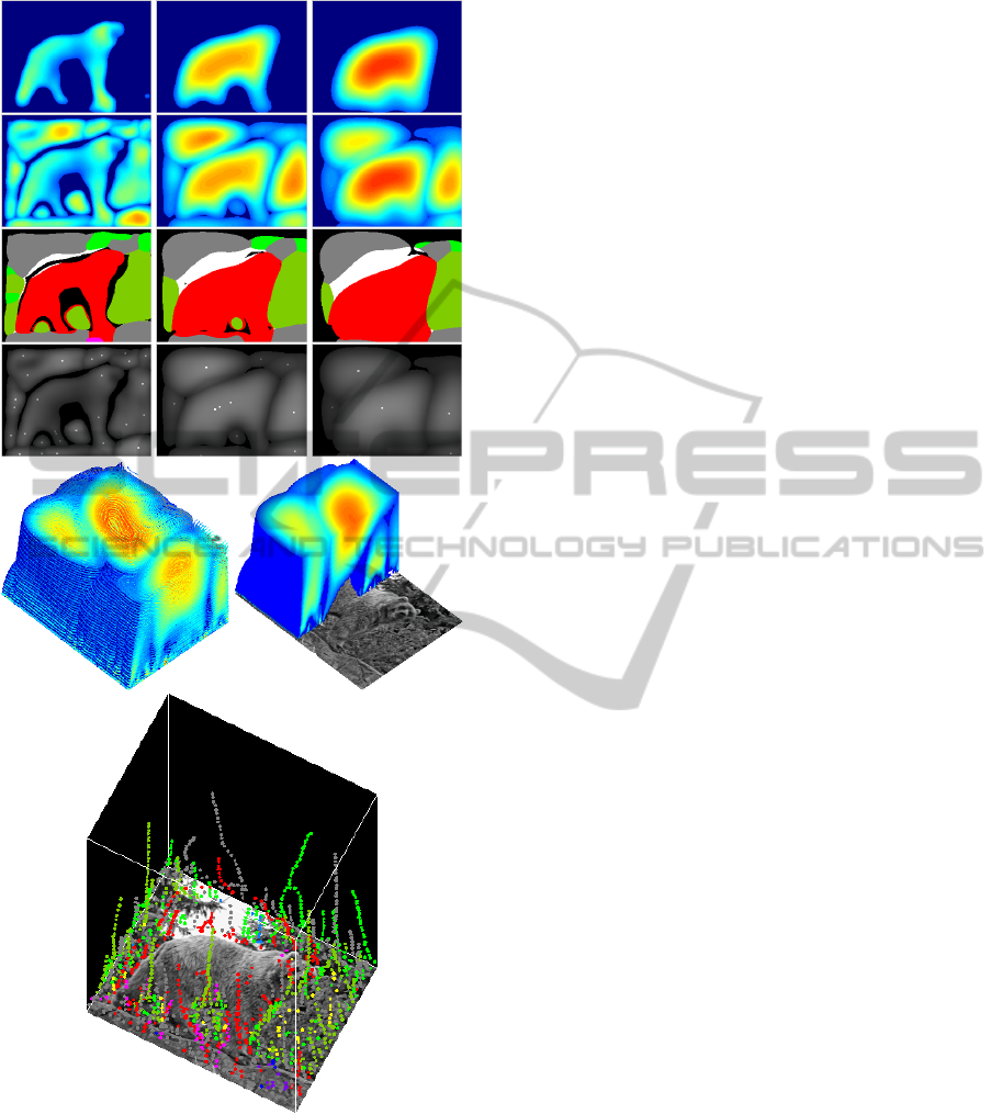
Figure 2: Top block: responses of colour double end-
stopped cells at, from left to right, three scales λ =
{12,24,32}. Top row:
ˆ
D
s,h
for φ
j
= 45
◦
. Second row:
˙
D
s
.
Third row: as 2nd row but with the corresponding hues φ
j
,
saturation in grey and luminance in white. Fourth row: ex-
trema E
D
s
superimposed on the combined responses of the
2nd row. At bottom: contours of the scale space (at left), a
cut shows the responses at successive scales (at right), and
linked extrema over scales with colour tags.
lenge, mainly because of different ranges of lengths
and forms. We tested several filters with different re-
ceptive field shapes and sizes, but because of com-
plexity and computational costs this solution was not
feasible.
Therefore we focused on the responses of oriented
double end-stopped cells, originally tuned to circu-
lar shapes, in order to also detect elongated shapes,
by combining them with the responses of completely
end-stopped cells for determining the length and ori-
entation of such regions. The method for region seg-
mentation consists of using such cells to cluster key-
points according to colour similarity and, by combin-
ing the clusters with the retinotopic colour maps and
line/edge maps, to detect region boundaries.
4.1 Keypoint Clustering
Keypoints of the same hue range φ
j
and at all scales
are combined into trees. We apply a multi-scale tree
structure in E
s
space, where one keypoint at a coarse
scale is related to one or more keypoints at one finer
scale, which can be slightly displaced. This relation
is modelled by down-projection using grouping cells
with a circular axonic field, the size of which (λ)
defines the region of influence; see (Farrajota et al.,
2011). Resulting trees, which are mainly caused by
responses of completely end-stopped cells, are then
separated from those caused by inhibited responses.
If a tree only comprises keypoints from “completely”
responses, it is considered to be a final cluster and it
is excluded from further processing.
The clustering consists of four steps: (1) Trees
of keypoints based on the E
s
space are assigned the
colour corresponding to the maximum response
˙
Λ
s
.
(2) Trees which mainly consist of keypoints where
at the same (x,y) position there exist inhibited com-
pletely end-stopped responses (CD = 0) are separated
from those with such non-inhibited responses – be-
cause inhibited responses are due to very elongated
regions whereas the other ones are due to circular or
semi-circular regions. (3) Trees with inhibited com-
pletely end-stopped responses in the same hue range
φ
j
are clustered on the basis of saturation, luminance
and spatial continuity. (4) The resulting clusters are
linked to other clusters which belong to neighbouring
hue ranges.
As mentioned, the clustering is divided in two
major groups: (a) more or less circular areas and
(b) elongated and differently shaped areas. In the
first case, we use the multi-scale keypoint trees (with
the same hue range φ
j
) in combination with com-
pletely end-stopped responses to detect and cluster
keypoints belonging to regions with different sur-
ICPRAM2014-InternationalConferenceonPatternRecognitionApplicationsandMethods
250

rounding regions, where keypoint trees at any scales
s which have inhibited completely end-stopped re-
sponses in any orientation were discarded, i.e., where
CD
s,i,h
(x,y)|
h=h
∗
= 0, where h
∗
corresponds to the
colour channel of the keypoints. The sizes of the re-
gions are directly related to the extrema with the high-
est responses, because the amplitudes of the responses
are directly related to the sizes of the RFs of com-
pletely double end-stopped cells. Therefore, a region
with an area which best fits a cell’s RF, at any given
scale, will yield the highest response of the keypoint
in the corresponding multi-scale tree for that particu-
lar region.
Elongated and differently shaped areas require
different clustering processes to ensure reliable de-
tection of the underlying colour patch and the clus-
tering of its features. After the first clustering
step in (2), keypoint trees with inhibited completely
end-stopped responses at any scale and orientation
(CD
s,i,h
(x,y)|
h=h
∗
= 0) are analysed and clustered to-
gether. Trees composed of extrema with inhibited re-
sponses of completely end-stopped cells, which be-
long to a same region, are clustered together using
saturation, luminance, colour range and spatial con-
nectivity. Let T
A
φ
and T
B
φ
be two trees with the
same colour φ. For each tree, the means
¯
C
∗
A
φ
=
∑
N
s
1
C
∗
(x,y)/N
s
and
¯
L
∗
A
φ
=
∑
N
s
1
L
∗
(x,y)/N
s
of the sat-
uration (chroma) and luminance channels are com-
puted, where N
s
is the number of scales of the tree.
If
¯
C
∗
A
φ
> 0.2 and
¯
L
∗
A
φ
> 0.25, then the spatial con-
nectivity is checked. A binary map B
j
is derived from
the colour maps CC
j
:
B
j
(x,y) =
(
1 if ψ
CC
j
(x,y) ≥ 0.7 ∧ ψ
SC(x,y)
≥ 0.7
0 otherwise.
(3)
Now, between two keypoints of the two trees and on a
straight line connecting the two extrema, if B
j
(x,y) =
0 at six or more consecutive positions on the line, the
link is considered invalid. If a valid link between all
pairs exists, the two trees are grouped together. This
process is repeated for all pairs of trees and tree clus-
ters, until all possible links have been checked.
Finally, tree clusters with all colours are evalu-
ated and possibly combined for the cases where the
hue of an underlying region lies between two colour
ranges. The ψ
SC
and ψ
L
channels are not included in
this step. In case of two clusters with neighbouring
colours φ
e
and φ
d
, where
|
e − d
|
≤ 1 and {e,d} ∈ j,
all pairs of trees between the clusters are compared as
in the previous clustering step, where the saturation
and luminance means are computed and validated. If
the validation is positive, the minimum distance of the
closest two keypoints in both trees is calculated, and
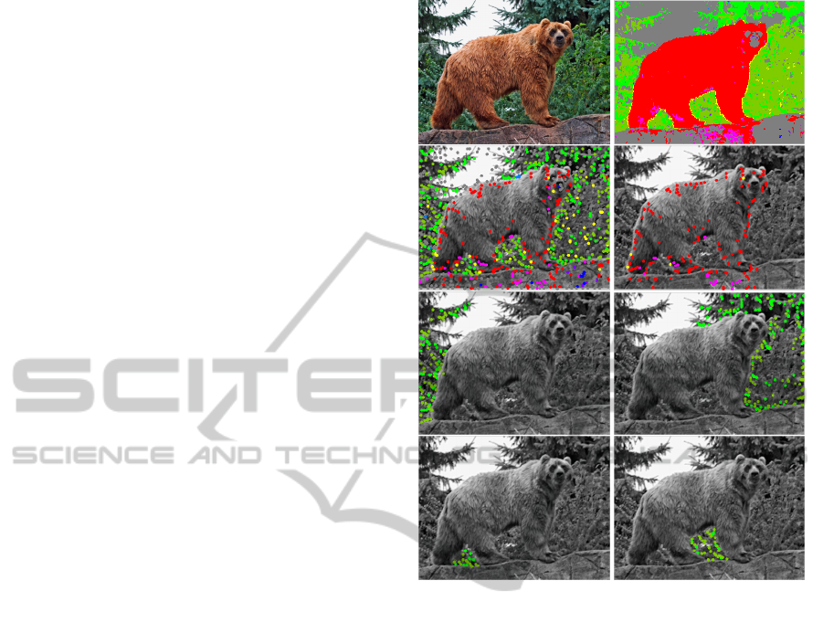
Figure 3: Clustering results. Top: input image (left) and
the maximum colour responses (right). Second row, left:
keypoints at all scales. Other images: examples of clustered
keypoints.
if the distance is less than 13 pixels (this was empir-
ically determined), both clusters are merged. In the
case of clusters which already contain two different
colour ranges (φ
e
, φ
d
), only clusters with those same
colour ranges are considered for validation and merg-
ing. As before, this process is repeated until no more
further links can be established. All trees which have
not been clustered with any other tree are discarded.
To avoid unnecessary computations and to speed
up the clustering process, responses of inhibited com-
pletely end-stopped cells of keypoints in multi-scale
trees are analysed with respect to inhibition of ori-
entations when comparing two extrema of two trees
or clusters of trees. For any orientation involved in
a keypoint from T
A
φ
with inhibited completely end-
stopped response (CD
s,i,h
= 0), if there exists a corre-
sponding orientation in a keypoint from T
B
φ
, then both
keypoints are valid candidates for spatial connectiv-
ity analysis. Invalid candidates are excluded from the
matching process.
Figure 3 shows examples of the clustering pro-
cess. The colours of the keypoints correspond to the
RegionSegregationbyLinkingKeypointsTunedtoColour
251

colour range φ
j
in H
∗
. The keypoints at all scales
(second row, left) serve to analyse the clustering re-
sults in the other images. In the bear (second row,
right) and in the left tree (third row, left) some key-
points are wrongly clustered (missing). In case of the
bear, the rock pigments near the right paw caused a
grouping because similar colours are too close spa-
tially. Such a problem cannot yet be solved. In case
of the left tree, some keypoints are missing (top left
corner) due to low saturation, which results in a sep-
arate cluster and which is not shown here. The areas
between the paws and rock are correctly clustered.
4.2 Segmentation
After keypoint clustering, a precise region segmenta-
tion must be achieved. Keypoint clusters are therefore
combined with an edge map and the colour maps. A
cluster’s coordinate boundaries are detected, a binary
map is obtained by combining the colour maps of the
colour (or colours) of the cluster with an edge map,
and all pixels inside the boundaries and the binary
map are extracted.
First, a region’s limits (bounding box) R =
{x
min
,y
min
,x
max
,y
max
} are retrieved from a cluster,
i.e., the keypoint positions at the cluster’s finest
scale, and a small relaxation is applied:
˙
R = {x
min
−
∆,y
min
− ∆,x
max
+ ∆,y
max
+ ∆}, with ∆ = 9 pixels.
This ensures that most if not all pixels from the re-
gion are included. Within this “window,” a binary
map which corresponds to the region’s colour cod-
ing is computed, such that any pixel within the same
colour ranges of the cluster in Γ(x,y) are 1 and all
others are 0.
Boundaries between regions are sometimes noisy
or badly defined due to camera focus, disparity, light-
ing, etc. An edge map is used to improve localisa-
tion. At a given (finest) scale s, the edge map EG
is constructed by combining responses of single end-
stopped cells in all orientations,
EG
s
(x,y) = max
h,i
(S
s,i,h
(x,y)). (4)
Only edges at the cluster’s finest scale are used
because of their better localisation. Then, non-
maximum suppression (NMS) is applied:
c
EG
s
=
NMS(EG
s
). This is done in all orientations in or-
der to preserve the peak responses of the best ori-
entations while suppressing weaker ones. Also, in
order to improve results, a hysteresis scheme like
(Canny, 1986) is applied, with thresholds T
low
= 0.2
and T
high
= 0.6. This ensures edge continuity. Fi-
nally, the edge map is binarised to 0 and 1.
The binary edge map is further refined by using
the colour maps. Pixels outside the boundaries de-
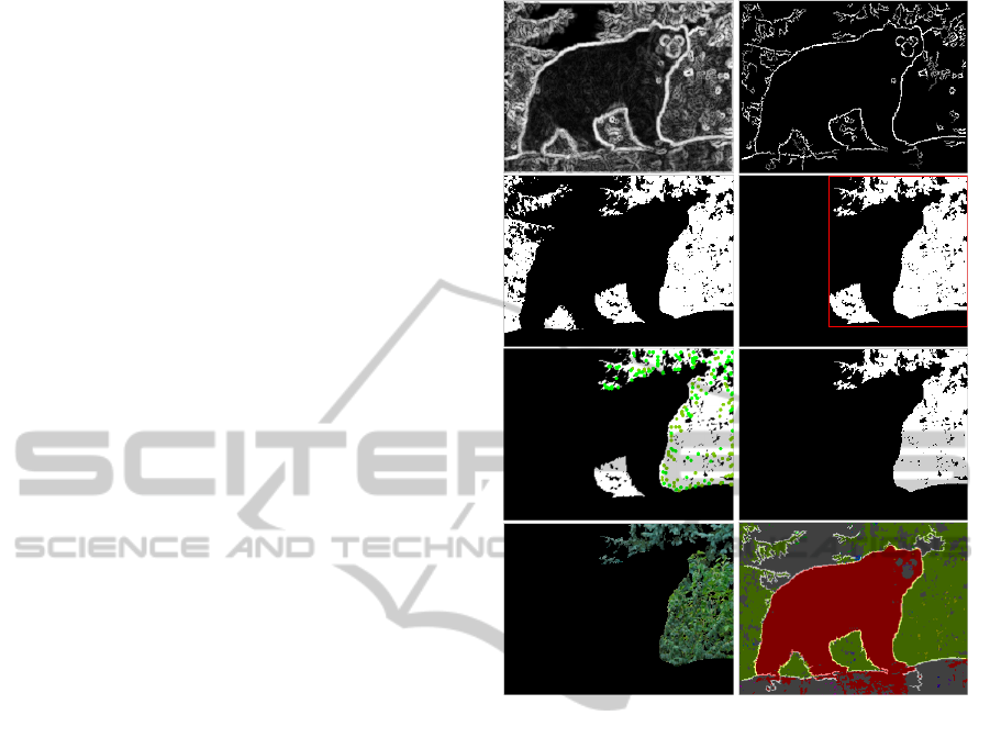
Figure 4: Segmentation results. Top row: edge maps
EG
s
|
s=1
before and after non-maximum suppression and
noise removal. Second and third row: the segmentation pro-
cess (see text). Fourth row: results (see text).
fined by the edge maps are considered to be outliers
which belong to other regions. These outliers are gen-
erally small sets of one or two pixels wide. Hence,
small sets of 5 pixels or less removed. Finally, a re-
gion is segmented by verifying whether the cluster’s
keypoint positions are contained in the binary map.
All regions without any keypoints contained in the re-
gions as defined by the clusters are inhibited.
Figure 4 illustrates the segmentation process and
shows results. The top row shows the edge maps ob-
tained from single end-stopped cells EG
s
at the finest
scale (left) and the result after non-maximum suppres-
sion and hysteresis tracking (right). On the second
row, the binary map (left) corresponds to the colours
of the cluster in Fig. 3 (third row, right). The re-
gion, delimited by the spatial positions of the com-
bined keypoints, i.e., the bounding box shown in red,
includes two separate regions (right). Then, by com-
bining the keypoint map with the edge map (third
row, left), the other region between the legs can be re-
moved (right). Finally, the region’s pixels in the input
image can be extracted (bottom-left), and all regions
ICPRAM2014-InternationalConferenceonPatternRecognitionApplicationsandMethods
252

can be shown and tagged by a number, including the
boundaries (bottom-right). Only big and meaningful
regions are shown in order to provide a clearer view
of the segmentation result.
5 CONCLUSIONS
In general, real-time computer vision requires huge
computational power because all images must be pro-
cessed from the first to the last pixel. GPU (graphics)
boards are becoming more popular as hardware ad-
vances, and more methods are being parallelised to
take advantage of massive parallelism. This concept
is fully employed by the primate visual system, in or-
der to execute complex visual tasks for real-time vi-
sion (Zeki, 1998). There is evidence that, like in the
macaque monkey, different areas of the human pre-
striate visual cortex are specialised for different vi-
sual attributes (Zeki et al., 1991; Grill-Spector and
Malach, 2004). Also, functional relationships were
discovered between areas V1/V2 and V4 in colour
vision, and between V1/V2 and V5 for motion pro-
cessing. These reflect the anatomical connections be-
tween these areas (Zeki et al., 1991). This indicates
that specialised neural processes for different tasks
also interact with each other, in both low-level (Li
et al., 2000) and high-level (Hansen and Gegenfurt-
ner, 2006) processes.
In this paper it has been shown that cortical cells
tuned to colour can be used to detect and segment re-
gions or patches according to their colour and shape.
Clusters of such regions can be used for higher-level
tasks such as object tracking and/or recognition. The
main advantage here is the high degree of parallelism:
most tasks can be performed simultaneously and inde-
pendently from each other. Also, resulting keypoints
from end-stopped cells code the local complexity of
a region, and their structure in a multi-scale tree in-
creases overall keypoint stability and speeds-up the
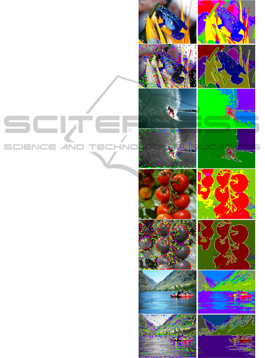
matching process (Farrajota et al., 2011). Results in
Fig. 5 show the applicability of the method to many
real images. On the 1st, 3rd, 5th and 7th rows it shows
the input image (left) and the maximum colour re-
sponses (right). The 2nd, 4th, 6th and 8th rows show
the keypoints at all scales (left) and the segmentation
results (right). As in Fig. 4 (fourth row, right), only
the most meaningful regions are shown for clarity.
The groupings of features in all images suggest that
meaningful regions can be obtained by the method,
and that these are suitable for higher-level tasks. By
combining colours and clusters of multi-scale key-
point trees, optical flow can be speeded up, not only
by direct tree matching but also by matching colour,
Figure 5: Segmentation results.
RegionSegregationbyLinkingKeypointsTunedtoColour
253

shape and size information. In addition, the cluster-
ing process can be optimised for recognising human
behaviour, because the parts of a person’s body can
be detected and coded by their shape and size over
time. This is crucial for recognising human gait, pos-
ture and gestures (Sminchisescu et al., 2011).
ACKNOWLEDGEMENTS
This work was supported by the EU under
the grant ICT-2009.2.1-270247 NeuralDynamics,
the Portuguese Foundation for LARSyS (PEst-
OE/EEI/LA0009/2013) and PhD grant to author MF
(SFRH/BD/79812/2011).
REFERENCES
Canny, J. (1986). A computational approach to edge detec-
tion. Pattern Analysis and Machine Intelligence, IEEE
Transactions on, (6):679–698.
Derrington, A. M., Parker, A., Barraclough, N. E., Easton,
A., Goodson, G. R., Parker, K. S., Tinsley, C. J., and
Webb, B. S. (2002). The uses of colour vision: be-
havioural and physiological distinctiveness of colour
stimuli. Phil. Trans. R. Soc. Lond. B, 357:975–985.
Farrajota, M., Rodrigues, J., and du Buf, J. (2011). Op-
tical flow by multi-scale annotated keypoints: A bi-
ological approach. Proc. Int. Conf. on Bio-inspired
Systems and Signal Processing (BIOSIGNALS 2011),
Rome, Italy, 26-29 January, pages 307–315.
Gegenfurtner, K. R. (2003). Cortical mechanisms of colour
vision. Nature Rev. Neurosci, 4:563–572.
Goddard, E., Mannion, D. J., McDonald, J. S., Solomon,
S. G., and Clifford, C. W. G. (2011). Color respon-
siveness argues against a dorsal component of human
v4. Journal of Vision, 11(4).
Grill-Spector, K. and Malach, R. (2004). The human visual
cortex. Annu. Rev. Neurosci., 27:649–677.
Grossberg, S., Mingolla, E., and Ross, W. D. (1997). Vi-
sual brain and visual perception: How does the cor-
tex do perceptual grouping? Trends in neurosciences,
20(3):106–111.
Hansen, T. and Gegenfurtner, K. R. (2006). Higher level
chromatic mechanisms for image segmentation. Jour-
nal of Vision, 6(3).
Hubel, D. (1995). Eye, Brain and Vision. Scientific Ameri-
can Library.
Jacobs, G. H. (2009). Evolution of colour vision in mam-
mals. Phil. Trans. R. Soc. B, 364:2957–2967.
Li, Z. et al. (2000). Pre-attentive segmentation in the pri-
mary visual cortex. Spatial Vision, 13(1):25–50.
Lucchese, L. and Mitra, S. (2001). Color image segmen-
tation: A state-of-the-art survey. Image Processing,
Vision, and Pattern Recognition, Proc. of the Indian
National Science Academy, 67(2):207–221.
Mushrif, M. M. and Ray, A. K. (2008). Color image seg-
mentation: Rough-set theoretic approach. Pattern
Recognition Letters, 29(4):483–493.
Pal, N. R. and Pal, S. K. (1993). A review on image segmen-
tation techniques. Pattern Recognition, 26(9):1277–
1294.
Robol, V., Casco, C., and Dakin, S. C. (2012)). The role of
crowding in contextual influences on contour integra-
tion. Journal of Vision, 12(7):1–18.
Rodrigues, J. and du Buf, J. (2006). Multi-scale keypoints
in V1 and beyond: object segregation, scale selection,
saliency maps and face detection. BioSystems, 2:75–
90.
Roe, A. W., Chelazzi, L., Connor, C. E., Conway, B. R.,
Fujita, I., Gallant, J. L., Lu, H., and Vanduffel, W.
(2012). Toward a unified theory of visual area v4.
Neuron, 74(1):12 – 29.
Shapley, R. and Hawken, M. (2011). Color in the cortex:
single- and double-opponent cells. Vision Research,
51:701–717.
Sminchisescu, C., Bo, L., Ionescu, C., and Kanaujia, A.
(2011). Feature-based pose estimation. In Visual
Analysis of Humans, pages 225–251. Springer.
Vantaram, S. R. and Saber, E. (2012). Unsupervised video
segmentation by dynamic volume growing and mul-
tivariate volume merging using color-texture-gradient
features. In Image Processing (ICIP), 19th IEEE In-
ternational Conference on, pages 305–308. IEEE.
Young, R. A., Lesperance, R. M., and Meyer, W. W. (2001).
The gaussian derivative model for spatial-temporal vi-
sion: I. cortical model. Spatial Vision, 14(3-4):261–
319.
Zeki, S. (1998). review: Parallel processing, asynchronous
perception, and a distributed system of consciousness
in vision. The Neuroscientist, 4(5):365–372.
Zeki, S., Watson, J., Lueck, C., Friston, K. J., Kennard, C.,
and Frackowiak, R. (1991). A direct demonstration of
functional specialization in human visual cortex. The
Journal of neuroscience, 11(3):641–649.
ICPRAM2014-InternationalConferenceonPatternRecognitionApplicationsandMethods
254