Use of Multiple Low Level Features to Find Interesting Regions

Michael Borck

1,2

, Geoff West

1,2

and Tele Tan

3,2

Department of Spatial Sciences, Curtin University, Perth, Australia

CRC for Spatial Information, Canberra, Australia

Department of Mechanical Engineering, Curtin University, Perth, Australia

Keywords:

Mobile Mapping, Feature Selection, Feature Extraction, Machine Learning, 3D Images.

Abstract:

Vehicle-based mobile mapping systems capture co-registered imagery and 3D point cloud information over

hundreds of kilometres of transport corridor. Methods for extracting information from these large datasets are

labour intensive and automatic methods are desired. In addition, such methods need to be easily conﬁgured

by non-expert users to detect and measure many classes of objects. This paper describes a workﬂow to take a

large number of image and depth features, use machine learning to generate an object detection system that is

fast to conﬁgure and run. The output is high detection of the objects of interest but with an acceptable number

of false alarms. This is desirable as the output is fed into a more complex and hence more computationally

expensive analysis system to reject the false alarms and measure the remaining objects. Image and depth

features from bounding boxes around objects of interest and random background are used for training with

some popular learning algorithms. The interface allows a non-expert user to observe the performance and

make modiﬁcations to improve the performance.

1 INTRODUCTION

Computer vision research is moving to the stage

where quite complex systems can be used in real

world applications, although in most cases the meth-

ods are turnkey. There are applications in which

a non-expert user needs to conﬁgure a complex se-

quence of processes for their application. Such an

application is the processing of co-registered imagery

and 3D point cloud information acquired from a mov-

ing vehicle along transport corridors. GPS and inertial

guidance allows the data to be registered to the world

coordinate system enabling reasonably accurate loca-

tion information to be acquired including the location

of street side furniture, width of roads, power line to

vegetation distances etc. Such systems can acquire

enormous amounts of data quite quickly. For exam-

ple the business district of Perth, Western Australia

consists of 320kms of roads resulting in 122GBytes

of image and depth data. Currently such data is pro-

cessed manually meaning it can take months to anal-

yse. The need is for methods to detect and measure

objects of interest to the user from the co-registered

imagery and depth data. Although 100% detection

with zero errors is desirable, however even if the per-

formance is such that less human intervention is spent

processing the data then that is a good outcome e.g.

100% detection and 20% false alarm rate.

This paper describes one stage of a multi-stage

system to speed up the processing of mobile map-

ping data. A large number of image and depth fea-

tures are extracted for objects of interest and the back-

ground. A number of classiﬁers are available that se-

lect the best combination of the features to give the

best performance. The parameters of the system can

be manipulated by the user to ﬁnd all the objects of

interest. The trade-off is a signiﬁcant number of false

alarms. However the overall result is that the number

of regions that have to be further analysed is reduced

meaning more complex and hence more computation-

ally intensive methods can be used to increase perfor-

mance. Results show that depth features improve the

performance over just image features.

Although the main objective is good detection per-

formance, the ease of use of such a system is also im-

portant, especially when integrated into the workﬂow

of the user. Use is made of Orange, a GUI based open

source interactive machine learning system (Dem

sar

et al., 2004). Modules have been written to carry out

image and depth processing and to interface to differ-

ent data providing systems.

The main data capturing system used was Earth-

654

Borck M., West G. and Tan T..

Use of Multiple Low Level Features to Find Interesting Regions.

DOI: 10.5220/0004827506540661

In Proceedings of the 3rd International Conference on Pattern Recognition Applications and Methods (ICPRAM-2014), pages 654-661

ISBN: 978-989-758-018-5

 2014 SCITEPRESS (Science and Technology Publications, Lda.)

mine, see Figure 1. The system captures panoramic

imagery and uses stereo algorithms to generate co-

registered 3D point clouds. Pairs of panoramic stereo

images are captured typically at 10 metre spacing

down a transport corridor. Each panorama is made

up of images from four cameras pointing to the front,

back, left and right of the vehicle. A 3D point cloud

surrounds the position of the cameras uses a stereo

template matching approach (Guinn, 2002).

Figure 1: Earthmine system showing two sets of panorama

cameras.

Earthmine has developed a server-based system

that allows the querying via location to obtain data

about a particular location. The data can be processed

using a number of methods e.g. randomly, from a

number of known locations, or by “driving” along the

capture pathway.

The paper has two main contributions. First, there

are questions on whether only image features or only

depth features or some combination of image and

depth should be used. Secondly the need to assess the

performance of feature selection and feature extrac-

tion on a variety of classiﬁers. Results are presented

that show the classiﬁcation performance of the sys-

tem on different objects and recommend appropriate

features and classiﬁers.

2 BACKGROUND

It is very easy for a non-expert user to select re-

gions from images using bounding boxes that iso-

late an object from the rest of the image. In most

cases bounding boxes add in background informa-

tion that can confuse recognition. Many features

have been proposed that have a certain amount of

“robustness” to the presence of background informa-

tion as well as attempting to allow a certain amount

of variation in the appearance of the object of inter-

est. Features such as Haar wavelets and Histogram

of Gradients (HoG) (Dalal and Triggs, 2005) have

proven popular. Descriptors can be dense or use in-

teresting points in the image. Some common in-

terest points descriptors include Scale-Invariant Fea-

ture Transform (SIFT) (Lowe, 2004), Speed Up Ro-

bust Features (SURF) (Bay et al., 2008) and Features

from Accelerated Segment Test (FAST) (Rosten et al.,

2010).

Similar to Alexe et al. (2010) it is assumed that an

object possess a uniqueness that allows it to be seg-

mented from the background and that this uniqueness

can be learned. This research differs with this and

other approaches as it includes the use of depth fea-

tures. The question is which combination of these de-

scriptors is best for each type of object that is required

to be detected? In essence the more features to select

from, the more likely the right combination will be

found. Some feature are tuned to different circum-

stances e.g. it is widely regarded that HoG is very

good for locating pedestrians but poor for other ob-

jects (Dalal and Triggs, 2005). Colour provides pow-

erful information for object detection but the RGB

channels are sensitive to lighting variations. In this

paper intensity, hue and saturation features will be

used. Statistical descriptors are quick to generate and

provide a compact representation.

Texture is another salient feature in images (He

and Wang, 1991). Textures have been described by

a precise statistical distribution of the image tex-

ture coming from the Gabor ﬁlter response (Wu

et al., 2001), local binary patterns (Zhao and

Pietikainen, 2006), and the Edge Histogram Descrip-

tor (EHD) (Wu et al., 2001). Mikolajczyk and Schmid

(2005) show that that moments and steerable ﬁlters,

like Gabor ﬁlters, show the best performance among

the low dimensional descriptors.

Interest points are often used to identify a point

in an image that may be useful in image match-

ing (Mikolajczyk and Schmid, 2001) and view-based

object recognition (Lowe, 2004). This research fo-

cuses on trying to recognise generic classes. The pro-

portion of interest points in a region is used as a de-

scriptor under the premise that interesting regions will

have a higher proportion of interest points.

Interesting regions will have more edges. It is not

always possible to obtain ideal edges so encoding the

proportion of edge pixels in a region is another mea-

sure to differentiate objects from non-objects (Phung

and Bouzerdoum, 2007). Alexe et al. (2010) examine

the edge density near the bounding box borders. In

this research both of these features are implemented.

A range image contains distance measurements

from a selected reference point or plane to surface

points of objects within a scene (Besl, 1988) allow-

ing more information of the scene to be recovered.

Simply extending available descriptors designed for

an intensity image to a depth image will not make use

of additional information encoded in the depth map.

Depth cues can improve object detection (Zhao et al.,

UseofMultipleLowLevelFeaturestoFindInterestingRegions

655

2012). It provides information about objects in terms

of geometry and shape (Badami et al., 2013). Fea-

ture extraction on range images has proven to be more

complex than on intensity images due to the irregular

distribution of range image data and the nature of the

features present in the range images (Coleman et al.,

2007).

Surface normals and curvature estimates are ex-

tremely fast and easy to compute, they approximate

the geometry of a point’s k-neighborhood with only

a few values. Similar to the orientation of edges, the

orientation of surface normals provide additional in-

formation about the object. Histogram of Oriented

Surface Normal (HoSN) (Tang et al., 2012) are de-

signed to capture local geometric characteristics for

object recognition with depth information. Local pla-

narity compares the planes of neighbourhood regions

by considering the relationship to the surrounding sur-

face normals (Cadena and Ko

secka, 2013)

Zhao et al. (2012) propose a local depth pattern as

a descriptor. They divide the region into cells, cal-

culate the average depth of each cell and then cal-

culate the difference between every cell pair. This

difference vector forms the descriptor. Cadena and

secka (2013) also use a depth difference feature

that is calculated on superpixels rather than cells.

3 WORKFLOW

In many applications of computer vision, workﬂow

is an important consideration. A user would typi-

cally read in some acquired data, process it inter-

actively and produce the desired result. Much em-

phasis is on manual control of the process. Simple

procedures can be fully automated if they are robust

enough. However for many recognition applications,

much tuning is needed by a skilled user. The chal-

lenge is to produce a workﬂow that a non-expert user

can use to conﬁgure a complex process such as ob-

ject detection. To do this, a user must be able to

view selected parts of the data, identify objects of in-

terest and train a system to use the best features for

recognition through a feature selection process com-

bined with some form of pattern recognition method

such as a decision tree. Such a system was build us-

ing Orange, an open source toolkit for machine learn-

ing onto which image processing, visualisation and

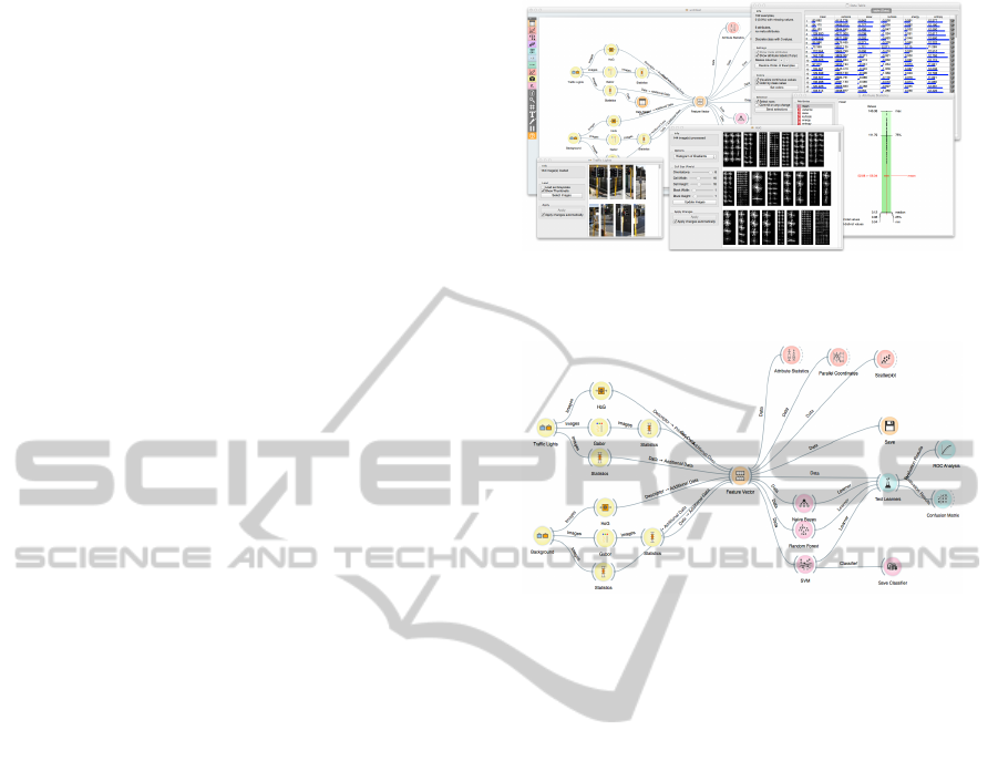
data acquisition methods were added. Figures 2 and

3 show an example of the workﬂow.

Figure 2: Example of image processing methods in Orange:

Histogram of Gradients and statistical measures.

Figure 3: Full workﬂow in Orange from data through to

classiﬁcation performance.

4 DATA

Our data consists of a pairs of co-registered RGB and

depth images. Within the Earthmine data set, 200 lo-

cations were visited. At each location each of the

front, back, left and right tile views were obtained and

bounding boxes deﬁned to select objects of interest

with the images. This resulted in a data set of 885 ex-

amples: 39 Bench seats; 53 Bus shelters; 69 Cars; 22

People; 81 Rubbish bins; 109 Street signs; 148 Trafﬁc

Lights; and 364 Background regions. Cars and people

are considered dead space and would be removed.

Some of the background regions were selected to

have similar aspect ratios to the objects as follows:

42 with aspect ratios similar to bus shelters; 93 with

aspect ratios similar to rubbish bins; 117 with aspect

rations similar to trafﬁc lights; and 112 regions of ran-

dom aspect ratios.

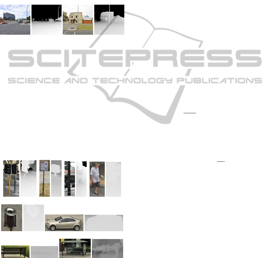
Figure 4 shows examples of intensity and depth

data from the Earthmine system. For each of the four

images: front, back, left and right, a depth image can

be generated that is co-registered with the intensity

image. In each of these images, darker pixels are fur-

ther from the cameras. The intensity images are typi-

cal of street scenes and captured at shutter speeds that

reduce blur as the vehicle could be travelling at 60-80

ICPRAM2014-InternationalConferenceonPatternRecognitionApplicationsandMethods

656

kmph. The depth images can be seen to correspond to

the intensity images especially with large scale parts

of the environment. Small scale objects are picked out

such as lamp posts. As with many stereo algorithms,

features such as edges are relied upon to give the best

estimation of depth from disparity and smooth areas

require interpolation between reliable depth estimates

to build a full depth map. The Earthmine data does

produce conﬁdence maps corresponding to the depth

data although they are not currently used in this work.

(a) (b)

Figure 4: Example pairs of co-registered intensity and depth

images (a) Image and depth map of an intersection. (b) Im-

age and depth map of building.

Figures 5(a) to 5(h) show examples of co-

registered intensity and depth images of the classes

of objects used for object recognition.

In some images there is noise and a lack of good

correspondence. Figure 5(a) shows a training image

for trafﬁc lights that have generally tall narrow bound-

ing boxes. Figure 5(h) shows some of the training im-

ages for bus shelters that have generally a more broad

aspect ratio. For all of these datasets, there is variation

in appearance of each object.

Randomly acquired background regions enables

the quick training of the system to discriminate be-

tween the objects of interest and the background.

(a) (b) (c) (d)

(e) (f)

(g) (h)

Figure 5: Example training image and corresponding depth

map for eight classes. (a) Trafﬁc light. (b) Street Sign. (c)

Background. (d) Person. (e) Rubbish Bin. (f) Car. (g)

Bench. (h) Bus Shelter.

5 FEATURES

For each bounding box a feature vector was con-

structed. For imagery intensity, hue and saturation

channels were used. For each channel the follow-

ing features are extracted: edge orientation histogram,

mean, variance, skew, kurtosis, energy, entropy, edge

density, Harris density, FAST density, local binary

pattern encoded as a normalised histogram, and Ga-

bor texture distribution encoded as mean and variance

for angles 0, 45, 90 and 135 degrees.

The features above were also computed on the

depth image when treated as a grey scale image. In

addition depth speciﬁc features mean curvature, local

planarity, an in-front-of feature, Histogram of Depth

Difference (HoDD) and Histogram of Surface Nor-

mals (HoSN) were calculated. These are explained

below.

Mean curvature was encoded as the mean and

variance of the curvature across the region. Equation

4 from Kurita and Boulanger (1992) was used to cal-

culate the curvature of a region.

Local planarity is computed using the dot product

between the normal to the local plane against the k-

neighbourhood normals:

1 −

k N k

∑

· n

j∈N

(1)

The in-front-of feature was encoded as the mean

and standard deviation of the Local Depth Difference

(LDD), where LDD is calculated between the depth

at a pixel, d

, and the k-neighbourhood’s depths, N:

LDD =

(

k d

− d

j∈N

k : d

kNk

∑

)

j∈N

0 : otherwise

(2)

To produce the HoDD, the region is divided into

cells of ﬁxed size. The difference of the average depth

values of every cell pair is then calculated. This dif-

ference is recorded as a ten bin histogram. The his-

togram is then normalised to allow comparison of dif-

ferent size image regions.

For HoSN, each pixel in the region had a plane ﬁt-

ted to the k-neighbouring pixels. The angle of surface

normal of the ﬁtted plane with respect to the vertical

plane was recorded in a histogram with bin size of

◦

. The normalised histogram was used as the fea-

ture vector.

6 EXPERIMENTAL PROCESS

The objective is to ﬁnd all objects of interest but with

manageable false alarm rate. To learn which fea-

UseofMultipleLowLevelFeaturestoFindInterestingRegions

657

tures and which classiﬁer performs the best a clas-

siﬁer pipeline is built. The pipeline is used to ex-

plore the performance using a training set consisting

of matching and non-matching image patches.

Classiﬁers considered include K-NN, N

aive

Bayes, Support Vector Machine (SVM), Decision

Trees, Random Forests, Boosting, Bagging and

Stacking. The last four are algorithms which use

multiple models to improve prediction performance.

Boosting and Bagging will be used to improve the

weakest classiﬁer identiﬁed during the preprocessing

phase. For the stacking classiﬁer all the classiﬁers ex-

cept SVM were combined. The implementation and

all details about these algorithms are available from

the Orange data mining system.

Performance of machine learning methods may

improve using a selected subset of best features. Fea-

ture selection is the process of selecting a subset of

relevant features for use in model construction (Mo-

toda and Liu, 2002). For this research a ﬁlter based

on SVM weights was used and a feature subset se-

lection wrapper based approach was written. The

bespoke wrapper uses forward search, an induction

algorithm, and search optimised for Area Under the

Curve (AUC).

An alternative is to use Principal Components

Analysis (PCA) to reduce the dimensionality of the

feature vector. Principal Components (PCs) are se-

lected by applying stopping rules (Jackson, 1993)

thereby reducing the dimensionality of the data. A

stopping rule is a decision criteria used to determine

how many PCs to use. Four stopping rules used in this

research include Kaiser-Guttman (Kaiser, 1960) and

Scree Plot (Jackson, 1993), Broken-Stick and vari-

ance covered.

A discretisation algorithm is used to handle prob-

lems with real-valued attributes with Decision Trees

and Bayesian Networks, treating the resulting inter-

vals as nominal values. Learners use the MDL-

Entropy discretisation method provided in the Orange

toolkit. For PCA and discretisation only the training

data is used to determine the transform. The learned

data transformation is applied to the test and valida-

tion data.

Half of the training data is used to tune classi-

ﬁers prior to conducting any experiments. The auto-

matic parameter search feature was used as provided

by the Orange machine learning software. If no au-

tomatic feature was provided the default parameters

were used. During this process a weak classiﬁer from

this initial process is identiﬁed to be used. On comple-

tion of tuning the parameters of each classiﬁer remain

ﬁxed for all of the experiments.

It is reasonable to expect different combinations

between feature representation and classiﬁers could

yield different performance. Classiﬁer Accuracy

(CA) and AUC are two popular measures used to

compare classiﬁers (Huang et al., 2003). Ling et al.

(2003) and Yan et al. (2003) show the AUC is sufﬁ-

cient when comparing classiﬁers.

However, selecting models based on best AUC

or CA can be misleading, especially if values are

close. Repeating experiments can often end up with a

slightly different values than previous runs. Method-

ologies are employed to reduce this effect, such as

cross validation, but cannot eliminate the effect. Sta-

tistical tests are conducted to determine if differences

in AUCs are statistically signiﬁcant. For classiﬁers

trained on the same data set the McNemar’s test is

used. McNemar’s test cannot be used on classiﬁers

trained on different data sets, so in this instance the

nonparametric Wilcoxon signed rank test is used.

7 RESULTS

A number of scenarios were explored for various

classiﬁers, classes and data sets. Data sets consid-

ered were image features, depth and a combination

of image and depth features. Prior to training, prin-

cipal components analysis and feature subset selec-

tion was applied to the data sets. A multiclass clas-

siﬁcation model was attempted to distinguish each on

the classes in the one model. Classiﬁers built were

based on K-NN, N

aive Bayes, SVM, Decision Tree

and Random Forest algorithm proved by the Orange

toolkit. For each dataset a 10-fold cross-validation

(using 70% of the data, 63:7) on each classiﬁer was

undertaken. Each classiﬁer is tested for CA and AUC

scores. Classiﬁers were ranked based on AUC and an

approximate best model selected. Preliminary anal-

ysis rejected many classiﬁers. Tables 1 - 3 show the

results for some of the better classiﬁers using different

feature sets.

For the experiments, the best AUC for image

features only was 0.967, 0.919 for depth features

only, and 0.978 for combined image and depth fea-

tures. The best classiﬁer is the Support Vector Ma-

chine. Similar performance was observed from Ran-

dom Forest classiﬁers (shown in bold in Tables 1-3).

Within each feature set four classiﬁers with the high-

est AUCs were selected for McNemar testing. Table 4

clearly shows that SVM was the best classiﬁer for the

Filter(20),image +depth data set (see Table 3)

The best classiﬁers from each data set were ranked

and a Wilcoxon signed rank test was performed pair-

wise on each set. For image features compared to

image and depth the mean p-value was 0.317 with

ICPRAM2014-InternationalConferenceonPatternRecognitionApplicationsandMethods

658

Table 1: Area Under Curve (AUC) and Classiﬁcation Accuracy (CA) for image features. The number in brackets indicates

how many features the classiﬁer used.

I+D (120) Filter (20) PCA (25) FSS-SVM (30)

Classiﬁer AUC CA AUC CA AUC CA AUC CA

Bayes 0.839 0.687 0.885 0.695 0.851 0.622 0.857 0.672

Tree 0.807 0.588 0.827 0.614 0.802 0.591 0.846 0.627

kNN 0.937 0.719 0.932 0.699 0.888 0.627 0.925 0.720

SVM 0.967 0.858 0.965 0.839 0.953 0.785 0.965 0.847

Forest 0.956 0.755 0.946 0.709 0.925 0.604 0.947 0.696

Stacked 0.949 0.776 0.935 0.724 0.914 0.661 0.940 0.727

Boosted 0.782 0.588 0.799 0.614 0.779 0.591 0.815 0.627

Bagged 0.910 0.722 0.907 0.698 0.890 0.677 0.910 0.733

Table 2: Area Under Curve (AUC) and Classiﬁcation Accuracy (CA) for depth features. The number in brackets indicates

how many features the classiﬁer used.

I+D (66) Filter (20) PCA (13) FSS-Bayes (27)

Classiﬁer AUC CA AUC CA AUC CA AUC CA

Bayes 0.818 0.538 0.800 0.474 0.825 0.474 0.815 0.490

Tree 0.767 0.531 0.741 0.490 0.777 0.474 0.735 0.489

kNN 0.899 0.599 0.826 0.520 0.824 0.485 0.847 0.539

SVM 0.918 0.661 0.919 0.644 0.898 0.590 0.911 0.628

Forest 0.910 0.598 0.852 0.528 0.841 0.443 0.881 0.543

Stacked 0.896 0.596 0.837 0.505 0.813 0.474 0.857 0.510

Boosted 0.739 0.531 0.708 0.490 0.693 0.474 0.712 0.489

Bagged 0.869 0.611 0.812 0.559 0.799 0.516 0.826 0.585

Table 3: Area Under Curve (AUC) and Classiﬁcation Accuracy (CA) for image and depth features. The number in brackets

indicates how many features the classiﬁer used.

I+D (186) Filter (20) PCA (25) FSS-kNN (34)

Classiﬁer AUC CA AUC CA AUC CA AUC CA

Bayes 0.823 0.678 0.886 0.687 0.876 0.656 0.877 0.695

Tree 0.815 0.615 0.841 0.617 0.796 0.546 0.839 0.646

kNN 0.962 0.767 0.936 0.711 0.898 0.643 0.953 0.769

SVM 0.978 0.859 0.975 0.843 0.971 0.813 0.978 0.855

Forest 0.969 0.773 0.952 0.706 0.936 0.606 0.960 0.743

Stacked 0.965 0.800 0.953 0.727 0.920 0.664 0.962 0.777

Boosted 0.811 0.615 0.812 0.617 0.767 0.546 0.812 0.646

Bagged 0.946 0.733 0.918 0.732 0.891 0.658 0.925 0.730

Table 4: McNemar table of top four classiﬁers from the im-

age and depth data set ﬁltered for top twenty ranked features

see column Filter(20) in Table 3.

McNemar > 3.84,5% Best

SVM vs Forest 57.366 Signiﬁcant SVM

SVM vs kNN 50.469 Signiﬁcant SVM

SVM vs Bagged 37.593 Signiﬁcant SVM

Forest vs kNN 0.043 Same neither

Forest vs Bagged 2.250 Same neither

kNN vs Bagged 1.190 Same neither

a standard deviation of 0.048. This indicates that

there was no signiﬁcant difference in discriminatory

performance between image and the combination of

depth and image. As there was no signiﬁcant differ-

ence in AUCs, Filter(20), SVM, image + depth with

the fewest number of features and better CA, was se-

lected as the overall best classiﬁer.

Using the best features, a Background vs Every-

thing classiﬁer was built to assess performance on

detecting any class from the background. Figure 6

shows ROC curves for different classiﬁers and is con-

sistent with previous results showing SVM, Random

Forest and N

aive Bayes being good classiﬁers.

8 CONCLUSIONS

This paper has detailed an investigation into the ﬁrst

stage of a system for recognising objects present in

UseofMultipleLowLevelFeaturestoFindInterestingRegions

659

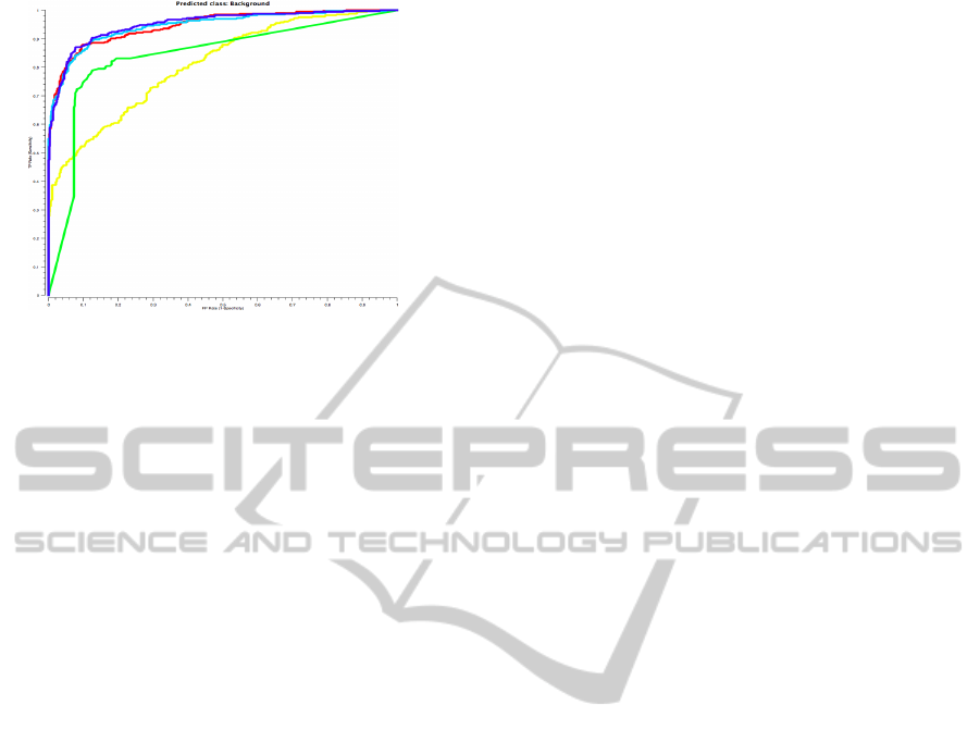
Figure 6: Background ROC curve for K-NN (Yellow), SVM

(Purple), Decision Tree (Green), Random Forest (Aqua)

and N

aive Bayes (Red).

co-registered image and depth data acquired from a

vehicle based mobile mapping system. The depth

data was acquired from the analysis of stereo pairs of

panoramic images with errors present that are com-

mon in stereo analysis. The methods used reﬂect the

need to ﬁnd a technique that a non-expert user can use

to train the system to do a relatively inexact recogni-

tion process to ﬁnd all the objects of interest with a

consequential signiﬁcant but manageable false alarm

rate. Bounding boxes are used to identify objects of

interest as well as random background examples for

training. A large number of features have been in-

vestigated with the thesis that machine learning will

select the most useful ones. Features have been ex-

plored from traditional RGB images as well as from

depth images using, in some cases, the same algo-

rithms by regarding the depth images as monochrome

grey scale images. The classiﬁcation results show that

image features perform better than depth features but

a combination of image and depth features performs

the best. The conclusion is that even quite coarse

depth features can improve performance.

Future work will explore larger feature sets for

each class, with more example classes. However it

has to be noted that, for training, the smallest number

of training examples is desired to improve the training

workﬂow for the user.

ACKNOWLEDGEMENTS

This work is supported by the Cooperative Research

Centre for Spatial Information, whose activities are

funded by the Australian Commonwealths Coopera-

tive Research Centres Programme. It provides PhD

scholarship for Michael Borck and partially funds

Professor Geoff West’s position. The authors would

like to thank John Ristevski and Anthony Fassero

from Earthmine and Landgate, WA for making avail-

able the datasets used in this work.

REFERENCES

Alexe, B., Deselaers, T., and Ferrari, V. (2010). What is

an object? Computer Vision and Pattern Recognition,

IEEE Computer Society Conference on.

Badami, I., St

uckler, J., and Behnke, S. (2013). Depth-

enhanced hough forests for object-class detection and

continuous pose estimation. Semantic Perception,

Mapping and Exploration, SPME-2013.

Bay, H., Ess, A., Tuytelaars, T., and Gool, L. V. (2008).

Speeded-up robust features (surf). Computer Vision

and Image Understanding, 110(3):346 – 359.

Besl, P. J. (1988). Active, optical range imaging sensors.

Machine vision and applications, 1(2):127–152.

Cadena, C. and Ko

secka, J. (2013). Semantic parsing for

priming object detection in rgb-d scenes. In Semantic

Perception, Mapping and Exploration (SPME) 2013.

Coleman, S., Scotney, B., and Suganthan, S. (2007). Fea-

ture extraction on range images - a new approach. In

Robotics and Automation, 2007 IEEE International

Conference on, pages 1098 –1103.

Dalal, N. and Triggs, B. (2005). Histograms of oriented

gradients for human detection. In Schmid, C., Soatto,

S., and Tomasi, C., editors, International Conference

on Computer Vision & Pattern Recognition, volume 2,

pages 886–893.

Dem

sar, J., Zupan, B., Leban, G., and Curk, T. (2004). Or-

ange: From experimental machine learning to interac-

tive data mining. In Boulicaut, J.-F., Esposito, F., Gi-

annotti, F., and Pedreschi, D., editors, Knowledge Dis-

covery in Databases: PKDD 2004, pages 537–539.

Springer.

Guinn, J. (2002). Enhanced formation ﬂying validation

report (jpl algorithm). NASA Goddard Space Flight

Center Rept, pages 02–0548.

He, D.-C. and Wang, L. (1991). Texture features based on

texture spectrum. Pattern Recognition, 24(5):391 –

399.

Huang, J., Lu, J., and Ling, C. (2003). Comparing naive

bayes, decision trees, and svm with auc and accuracy.

In Data Mining, 2003. ICDM 2003. Third IEEE Inter-

national Conference on, pages 553–556.

Jackson, D. A. (1993). Stopping rules in principal compo-

nents analysis: a comparison of heuristical and statis-

tical approaches. Ecology, pages 2204–2214.

Kaiser, H. F. (1960). The application of electronic comput-

ers to factor analysis. Educational and psychological

measurement.

Kurita, T. and Boulanger, P. (1992). Computation of sur-

face curvature from range images using geometrically

intrinsic weights. MVA, pages 389–392.

Ling, C. X., Huang, J., and Zhang, H. (2003). Auc: a bet-

ter measure than accuracy in comparing learning al-

gorithms. In Advances in Artiﬁcial Intelligence, pages

329–341. Springer.

ICPRAM2014-InternationalConferenceonPatternRecognitionApplicationsandMethods

660

Lowe, D. G. (2004). Distinctive image features from scale-

invariant keypoints. International Journal of Com-

puter Vision, 60(2):91–110.

Mikolajczyk, K. and Schmid, C. (2001). Indexing based

on scale invariant interest points. In Proceedings of

Eighth IEEE International Conference on Computer

Vision, 2001., volume 1, pages 525 –531.

Mikolajczyk, K. and Schmid, C. (2005). A perfor-

mance evaluation of local descriptors. IEEE Trans-

actions on Pattern Analysis & Machine Intelligence,

27(10):1615–1630.

Motoda, H. and Liu, H. (2002). Feature selection, extrac-

tion and construction. Communication of IICM (In-

stitute of Information and Computing Machinery, Tai-

wan) Vol, 5:67–72.

Phung, S. and Bouzerdoum, A. (2007). Detecting people

in images: An edge density approach. In Acoustics,

Speech and Signal Processing, 2007. ICASSP 2007.

IEEE International Conference on, volume 1, pages

I–1229 –I–1232.

Rosten, E., Porter, R., and Drummond, T. (2010). Faster and

better: A machine learning approach to corner detec-

tion. Pattern Analysis and Machine Intelligence, IEEE

Transactions on, 32(1):105 –119.

Tang, S., Wang, X., Lv, X., Han, T. X., Keller, J., He,

Z., Skubic, M., and Lao, S. (2012). Histogram of

oriented normal vectors for object recognition with a

depth sensor. In Proceedings of 11th Asian Confer-

ence on Computer Vision (ACCV 2012).

Wu, P., Ro, Y., Won, C., and Choi, Y. (2001). Texture

descriptors in mpeg-7. In Skarbek, W., editor, Com-

puter Analysis of Images and Patterns, volume 2124

of Lecture Notes in Computer Science, pages 21–28.

Springer Berlin Heidelberg.

Yan, L., Mozer, M. C., and Wolniewicz, R. (2003). Opti-

mizing classiﬁer performance via an approximation to

the wilcoxon-mann-whitney statistic. Proceedings of

the 20th International Conference on Machine Learn-

ing.

Zhao, G. and Pietikainen, M. (2006). Local binary pat-

tern descriptors for dynamic texture recognition. In

Pattern Recognition, 2006. ICPR 2006. 18th Inter-

national Conference on, volume 2, pages 211–214.

IEEE.

Zhao, Y., Liu, Z., Yang, L., and Cheng, H. (2012). Comb-

ing rgb and depth map features for human activity

recognition. In Signal Information Processing As-

sociation Annual Summit Conference (APSIPA ASC),

2012 Asia-Paciﬁc, pages 1–4.

UseofMultipleLowLevelFeaturestoFindInterestingRegions

661