
Kernel Hierarchical Agglomerative Clustering
Comparison of Different Gap Statistics to Estimate the Number of Clusters
Na Li, Nicolas Lefebvre and R´egis Lengell´e
Charles Delaunay Institute - UMR CNRS 6281, Universit´e de Technologie de Troyes, 12 Rue Marie Curie, Troyes, France
Keywords:
Hierarchical Agglomerative Clustering, Gap Statistics, Kernel Alignment, Number of Clusters.
Abstract:
Clustering algorithms, as unsupervised analysis tools, are useful for exploring data structure and have owned
great success in many disciplines. For most of the clustering algorithms like k-means, determining the number
of the clusters is a crucial step and is one of the most difficult problems. Hierarchical Agglomerative Clustering
(HAC) has the advantage of giving a data representation by the dendrogram that allows clustering by cutting
the dendrogram at some optimal level. In the past years and within the context of HAC, efficient statistics have
been proposed to estimate the number of clusters and the Gap Statistic by Tibshirani has shown interesting
performances. In this paper, we propose some new Gap Statistics to further improve the determination of the
number of clusters. Our works focus on the kernelized version of the widely-used Hierarchical Clustering
Algorithm.
1 INTRODUCTION
Clustering is the task of grouping objects according to
some measured or perceived characteristics of them
and it has owned great success in exploring the hid-
den structure of unlabeled data sets. As a useful tool
for unsupervised classification, it has drawn increas-
ing attention in various domains including psychol-
ogy (Harman, 1960), biology (Sneath et al., 1973) and
computer security (Barbar´a and Jajodia, 2002). Clus-
tering algorithms have a long history. They originated
in anthropology by Driver and Kroeber (Driver and
Kroeber, 1932). In 1967 one of the most useful and
simple clustering algorithms, k-means (Mac Queen
et al., 1967), has been proposed. Since then a lot
of classical algorithms, like fuzzy c-means (Bezdek
et al., 1984), Hierarchical Agglomerative Clustering
(HAC) etc have emerged.
Meanwhile, another clustering method, kernel-
based clustering, has arisen and owned great success
because of its ability to perform linear tasks in some
non linearly transformed spaces. In machine learn-
ing, the kernel trick has been firstly introduced by
Aizerman (Aizerman et al., 1964). It became fa-
mous in Support Vector Machines (SVM) initially
proposed by Cortes and Vapnik (Cortes and Vapnik,
1995). SVM has shown better performances in many
problems and this success has brought an extensive
use of the kernel trick into other algorithms like ker-
nel PCA (Sch¨olkopf et al., 1998), non linear (adap-
tive) filtering (Pr´ıncipe et al., 2011) etc. Kernel meth-
ods have been widely used in supervised classifica-
tion tasks like SVM and then they were extended to
unsupervised classification. A lot of kernel-induced
clustering algorithms have emerged due to the exten-
sive use of inner products. Most of these algorithms
are kernelized versions of the corresponding conven-
tional algorithms. Surveys of kernel-induced meth-
ods for clustering have been done in (Filippone et al.,
2008; Kim et al., 2005; Muller et al., 2001). The first
proposed and the most well-known kernel-induced al-
gorithm is kernel k-means by Scholkopf (Sch¨olkopf
et al., 1998). A further version has been proposed
by Girolami (Girolami, 2002). After that, several
kernel-induced algorithms have emerged such as ker-
nel fuzzy c-means, kernel Self Organizing Maps, ker-
nel average-linkage etc. Compared with the corre-
sponding conventional algorithms, kernelized criteria
have shown better performance especially for non-
linearly separable data sets.
According to our literature survey, a few work has
been done on kernel based HAC (see, e.g. (Qin et al.,
2003), (Kim et al., 2005)). The prominence of HAC
consists in the data description provided by a den-
drogram which represents a tree of nested partitions
of the data. Hierarchical clustering usually depends
on distance calculations (to compute between-class
and within-class dispersions, minimum linkage, max-
255
Li N., Lefebvre N. and Lengellé R..
Kernel Hierarchical Agglomerative Clustering - Comparison of Different Gap Statistics to Estimate the Number of Clusters.
DOI: 10.5220/0004828202550262
In Proceedings of the 3rd International Conference on Pattern Recognition Applications and Methods (ICPRAM-2014), pages 255-262
ISBN: 978-989-758-018-5
Copyright
c
2014 SCITEPRESS (Science and Technology Publications, Lda.)

imum linkage etc) which are based on inner products.
In order to explore wider classes of classifiers, we
can perform HAC after mapping the input data onto a
higher dimension space using a nonlinear transform.
This is one of the main ideas of kernel methods, where
the transformed space is selected as a Reproducing
Kernel Hilbert Space (RKHS) in which distance cal-
culations can be easily evaluated with the help of the
kernel trick (Aizerman et al., 1964).
In this paper we focus on the kernel based HAC
framework which is robust in clustering non linearly
separable data sets and, at the same time, several cri-
teria are proposed to determinate the number of clus-
ters, being inspired by the Gap Statistic of Tibshirani
(Tibshirani et al., 2001). This paper is organized as
follows: we start with an introduction of kernel HAC.
Then we introduce the principle of Gap Statistics and
our criteria to estimate the number of clusters. Subse-
quently, we provide the results of a simulation study
and we compare the results obtained with those of
Tibshirani, in standard and kernel HAC. We show that
alternate Gap Statistics are possible to estimate the
number of clusters and one of them, the Delta Level
Gap, is efficient and robust to variations in the cluster-
ing procedure. Finally, we propose some perspectives
to this work in order to obtain a fully automatic clus-
tering algorithm.
2 KERNEL HIERARCHICAL
AGGLOMERATIVE
CLUSTERING (K-HAC)
2.1 Kernel Trick
The key notion in kernel based algorithms is the ker-
nel trick. To introduce the kernel trick, we first re-
call Mercer’s theorem (Mercer, 1909). Let X be the
original space. A kernel function K : X × X −→ R is
called a positive definite kernel (or Mercer Kernel) if
and only if:
• K is symmetric: K(x,y) = K(y,x) ∀(x, y) ∈ X ×X
•
∑
n
i=1
∑
n
j=1
c
i
c
j
K(x
i
,x
j
) ≥ 0, ∀i = 1,...,n,∀n ≥ 2
where c
i
∈ R
For each Mercer kernel we have:
K(x
i
,x
j
) = hΦ(x
i
),Φ(x
j
)i (1)
where φ : X → F performs the mapping from the orig-
inal space onto the (high dimensional) feature space.
As shown in equation (1), inner product calculations
in the feature space can be computed by a kernel func-
tion in the original space, without explicitly speci-
fying the mapping function Φ. The computation of
Euclidean distance in feature space F benefits from
this idea.
d
2
(Φ(x
i
),Φ(x
j
)) = kΦ(x
i
) − Φ(x
j
)k
2
(2)
= K(x
i
,x
i
) + K(x
j
,x
j
) − 2K(x
i
,x
j
)
Several commonly used Mercer kernels are listed
in (Vapnik, 2000). In this paper, we only consider the
gaussian kernel defined as follows:
K(x
i
,x
j
) = exp
−
k x
i
− x
j
k
2
2σ
2
(3)
2.2 Kernel-HAC
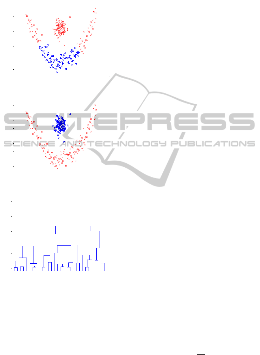
The advantage of HAC lies in the obtention of den-
drogram (see an example in Figure 3), which gives a
description of the data structure. By cutting the den-
drogramat a givenlevel, one can perform data cluster-
ing. The aim of introducing the kernel trick in HAC
is to easily explore wider classes of similarity mea-
sures. Figures 1 and 2 show an example of a data set
that cannot be clustered by standard HAC (Figure 1)
while kernel HAC allows perfect clustering (Figure
2).
The HAC algorithm steps are 1) assign each data
point to be a singleton; 2) calculate some similar-
ity/dissimilarity between each pair of clusters; 3)
merge the pairwise closest clusters into one; 4) repeat
the two previous steps until only one final cluster is
obtained.
Different similarity measures have been proposed
and surveys have been done in (Murtagh, 1983; Ol-
son, 1995). Examples of linkage criteria are:
• Single linkage
d(r,s) = min(d(x
ri
,x
rj
)), x
ri
∈ r, x
rj
∈ s
• Complete linkage
d(r,s) = max(d(x
ri
,x
rj
)), x
ri
∈ r, x
rj
∈ s
• Average linkage
d(r,s) =
1
n
r
n
s
∑
n
r
i=1
∑
n
s
j=1
d(x
ir
,x
js
)
• Ward’s linkage
d
2
(r, s) = n
r
n
s
k ¯x
r
− ¯x
s
k
2
2
(n
r
+n
s
)
In this paper, we focus on the gaussian kernel
based HAC using Ward’s linkage criterion. In Ward’s
linkage, ¯x
r
denotes the the centroid of cluster r, ¯x
r
=
1
n
r
∑
n
r
i
x
i
. So in the feature space F, we have:
d
2
(r
Φ
,s
Φ
) =
n
r
n
s
(n
r
+ n
s
)
1
n
2
r
n
r
∑
i
n
r
∑
j
K(x
i
,x
j
)
+
1
n
2
s
n
s
∑
i
n
s
∑
j
K(x
i
,x
j
) −
2
n
r
n
s
n
r
∑
i
n
s
∑
j
K(x
i
,x
j
)
!
(4)
ICPRAM2014-InternationalConferenceonPatternRecognitionApplicationsandMethods
256
−3 −2 −1 0 1 2 3
−2.5
−2
−1.5
−1
−0.5
0
0.5
1
1.5
2
2.5
Figure 1: Result using HAC.
−3 −2 −1 0 1 2 3
−2.5
−2
−1.5
−1
−0.5
0
0.5
1
1.5
2
2.5
Figure 2: Result using kernel HAC.
11292613 4 11230 7 2201628 6 81517212223 3 924182725 5191014
1
2
3
4
5
6
7
8
9
10
Figure 3: Dendrogram of this data set using kernel HAC.
As can be seen in figures 1 and 2 kernel HAC
allows clustering of separable classes with small
between-class dispersion in the original space.
3 DETERMINING THE NUMBER
OF CLUSTERS
Determining the number of clusters is one of the most
difficult problems in cluster analysis. For some algo-
rithms like k-means, the number of clusters needs to
be provided in advance. Over the past years, a lot of
methods have emerged and the Gap Statistic proposed
by Tibshirani (Tibshirani et al., 2001) is probably one
of the most promising approach.
In the earlier times, Milligan and Copper (Milli-
gan and Cooper, 1985) have done a research on the
criteria for estimating the number of clusters, report-
ing the results of a simulation experiment designed
to determine the validity of 30 criteria proposed in
the literature. After that, several criteria emerged
like Hartigan’s rule (Hartigan, 1975), Krzanowski and
Lai’s index (Krzanowski and Lai, 1988), the silhou-
ette statistic suggested by Kaufman and Rousseeuw
(Kaufman and Rousseeuw, 2009) and Calinski and
Harabasz’s index (Cali´nski and Harabasz, 1974),
which has demonstrated better performance under
most of the situations considered in Milligan and
Copper’s study. More recent methods on determin-
ing the number of clusters include an approach using
approximate Bayes factors proposed by Fraley and
Raftery (Fraley and Raftery, 1998) and a jump method
by Sugar and James (Sugar and James, 2003).
Unfortunately, most of these methods are some-
what ad hoc or model-based and hence sometimes re-
quire parametric assumptions which lead to a lack of
generality. However, the principle of Gap Statistics
proposed by Tibshirani et al. (Tibshirani et al., 2001)
is to compare the within cluster dispersion obtained
by the considered clustering algorithm with that we
would obtain under a single cluster hypothesis. It is
designed to be applicable to virtually any clustering
method like the commonly used k-means and HAC.
3.1 Gap Statistics
Consider a data set x
ij
,i = 1,2,...,n, j = 1,2,..., p,
consisting of p features, all of them being measured
on n independent observations. d
ii
′
denotes some dis-
similarity between observations i and i
′
. The most
common used dissimilarity measure is the squared
Euclidean distance (
∑
j
(x
ij
− x
i
′
j
)
2
). Suppose that the
data set is composed of k clusters and that C
r
denotes
the indices of observations in cluster r and n
r
= |C
r
|.
According to Tibshirani, and using his notations, we
define:
D
r
=
∑
i,i
′
∈C
r
d
ii
′
(5)
as the sum of all the distances between any two ob-
servations in cluster r. So, using again the notations
of Tibshirani,
W
k
=
k
∑
r=1
1
2n
r
D
r
(6)
KernelHierarchicalAgglomerativeClustering-ComparisonofDifferentGapStatisticstoEstimatetheNumberofClusters
257
is the within-class dispersion. W
k
monotonically de-
creases as the number of clusters k increases but, ac-
cording to Tibshirani (Tibshirani et al., 2001), from
some k onwards, the rate of decrease is dramatically
reduced. It has been shown that the location of such
an elbow indicates the appropriate number of clusters.
The main idea of Gap Statistics is to compare the
graph of log(W
k
) with its expectation we could ob-
serve under a single cluster hypothesis (the impor-
tance of the choice of an appropriate null reference
distribution of the data has been studied in (Gordon,
1996)).
According to (Tibshirani et al., 2001), the as-
sumed null model of the data set must be a single
cluster model. The most common considered refer-
ence distributions are:
• an uniform distribution over the range of the ob-
served data set.
• an uniform distribution over an area which is
aligned with the principal components of the data
set.
The first method has the advantage of simplicity
while the second is more accurate in terms of consis-
tency because it takes into account the shape of the
data distribution.
Here again, using the notations of Tibshirani, we
define the Gap Statistic as:
Gap(k) = E
n
{log(W
k
/H
0
)} − log(W
k
) (7)
Here E
n
{log(W
k
/H
0
)} denotes the expectation of
log(W
k
) under some null reference distribution H
0
.
The estimated number of clusters
ˆ
k falls at the point
where Gap
n
(k) is maximum. Expectation is esti-
mated by averaging the results obtained from differ-
ent realizations of the data set under the null reference
distribution.
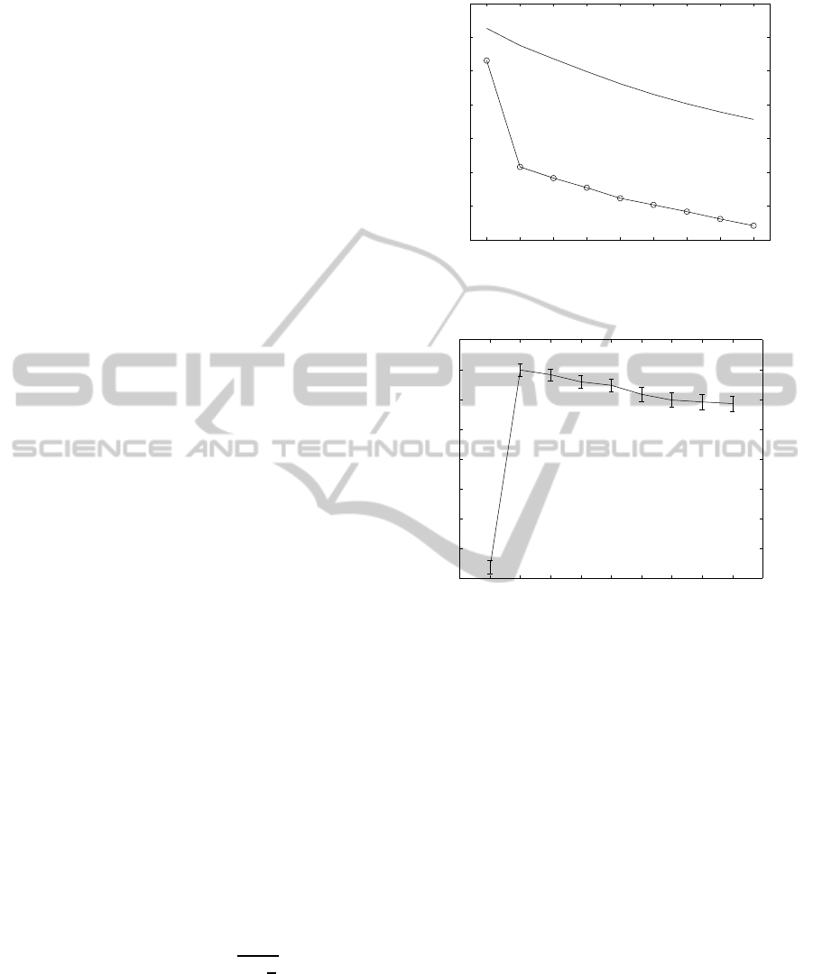
Figures 4 and 5 show an example using ker-
nel HAC. Data are composed of three distinct bi-
dimensional Gaussian clusters centred on (0, 0),
(0,1.3), (1.4,−1) respectively, with unit covariance
matrix I
2
and 100 observations per class. The func-
tions log(W
k
) and the estimate of E
n
{log(W
k
/H
0
)}
are shown in Figure 4. The Gap Statistic is shown
in Figure 5. In this example, E
n
{log(W
k
/H
0
)} was
estimated using 150 independent realizations of the
null data set. We also estimated the standard deviation
sd(k) of log(W
k
/H
0
). Let s
k
=
q
1+
1
B
sd(k), which
is represented by vertical bars in Figure 5, then, ac-
cording to Tibshirani, the estimated number of cluster
ˆ
k is the smallest k such that:
Gap(k) ≥ Gap(k + 1) − s
k+1
(8)
Figure 5 shows that, for the considered data set,
ˆ
k = 3,
which is correct.
2 3 4 5 6 7 8 9 10
1.5
2
2.5
3
3.5
4
4.5
5
E
E
E
E
E
E
E
E
E
Number of clusters k
Obs and Exp log(W
k
)
Figure 4: Graphs of E
n
{log(W
k
/H
0
)} (upper curve) and
log(W
k
) (lower curve).
1 2 3 4 5 6 7 8 9 10 11
0.4
0.6
0.8
1
1.2
1.4
1.6
1.8
2
Number of clusters k
Figure 5: Gap statistic as a function of the number of clus-
ters.
3.2 New Criteria to Estimate the
Number of Clusters in Kernel HAC
The main idea of Gap Statistics was to compare the
within-class dispersion obtained on the data with that
of an appropriate reference distribution. Inspired by
this idea, we propose to extend it to other criteria
which are suitable for HAC to estimate the number
of clusters.
These criteria are:
• Modified Gap Statistic
In the Gap Statistic proposed by Tibshirani, the
estimated number of clusters
ˆ
k is chosen accord-
ing to equation 8. In this modified Gap Statis-
tic, we define
ˆ
k as the number of clusters where
Gap(k) (equation 7) is maximum. As will be
shown later in this paper, this allows to potentially
improve the estimate, at least for standard HAC.
• Centered Alignment Gap
A good guess for the nonlinear function Φ(x
i
)
should be to directly produce the expected result
ICPRAM2014-InternationalConferenceonPatternRecognitionApplicationsandMethods
258

y
i
for all observations. In this case, the best Gram
matrix K whose general term is K
ij
= K(x
i
,x
j
)
becomes YY
′
where Y is the column vector (or
matrix, depending on the selected code book) of
all the data labels. Shawe-Taylor et al. ((Shawe-
Taylor and Kandola, 2002)) have proposed a func-
tion that depends on both the labels and the Gram
matrix, called alignment, to measure the degree
of agreement between a kernel function and the
clustering task. The alignment is defined by:
Alignment =
< K,YY
′
>
F
p
< K,K >
F
< YY
′
,YY
′
>
F
(9)
where the subscript F denotes Frobenius norm. In
this paper, Y is estimated after the clustering pro-
cess. The Centered Alignment (CA) is defined as:
CA =
< K
c
,Y
c
Y
c
′
>
F
p
< K
c
,K
c
>
F
< Y
c
Y
c
′
,Y
c
Y
c
′
>
F
(10)
Here the centered matrix K
c
associated to the ma-
trix K is defined by:
K
c
(x,y) = hΦ(x) − E
x
[Φ],Φ(x
′
) − E
x
′
[Φ]i
= K(x,y) − E
x
[K(x,y)] − E
y
[K(x,y)]
+E
x,y
[K(x,y)]
where the expectation operator is evaluated by av-
eraging over the data. Y
c
is defined by:
Y
c
= Y − E[Y]
So the Centered Alignment Gap is defined by:
Gap
CA
(k) = E
n
{CA/H
0
} −CA (11)
The estimated number of clusters
ˆ
k is the k such
that Gap
CA
(k) is maximum.
• Delta Level Gap
In the dendrogram, we consider each level of the
similarity measure h
i
,i = 1...n − 1 where h
1
is
the highest level. Then we define ∆h(k) = h
i
−
h
i+1
,k = 2...n. We define the criterion Delta Level
Gap:
Gap
∆h(k)
(k) = ∆h(k) − E
n
{∆h(k)/H
0
} (12)
The estimated number of clusters
ˆ
k is the value of
k where Gap
∆h(k)
(k) is maximum.
• Weighted Delta Level Gap
This criterion is related to the previous one.
We define the Weighted Delta Level (denoted
by ∆h
W
(k)) by: ∆h
W
(2) = ∆h(2),k = 2 and
∆h
W
(k) =
∆h(k)
∑
k−1
i=2
∆h(i)
,k ≥ 2. We define the criterion
Weighted Delta Level Gap as:
Gap
∆h
W
(k)
(k) = ∆h
W
(k) − E
n
{∆h
W
(k)/H
0
}
(13)
The estimated number of clusters
ˆ
k is the value of
k where Gap
∆h
W
(k)
(k) is maximum.
4 SIMULATIONS
We have generated 6 different data sets to compare
the proposed criteria with that from Tibshirani:
1. Five clusters in two dimensions
(1)
The clusters consist of gaussian bidimensional
distributions N(0,1.5
2
) centered at (0,0), (-3,3),
(3,-3), (3,3) and (-3,-3). Each cluster is composed
of 50 observations. Clusters strongly overlap. The
kernel parameter is σ = 0.90.
2. Five clusters in two dimensions
(2)
The data are generated in the same way as in the
previous case but the variance of the clusters is
now 1.25
2
). Clusters slightly overlap. σ = 0.85.
3. Five clusters in two dimensions
(3)
Same case but with variance equal to 1.0
2
. There
is no overlap. σ = 0.80.
4. Three clusters in two dimensions
This is a data set used by Tibshirani (Tibshirani
et al., 2001). The clusters are unit variance gaus-
sian bidimensional distributions with 25,25,50
observations, centered at (0, 0), (0,5) and (5,−3),
respectively. σ = 0.80.
5. Two nested circles and one outside isolated disk
in two dimensions
These three circles are centered at (0,0), (0,0)
and (0, 8) with 150, 100,100 observations. The
respective radii are uniformly distributed over
[0,1], [4,5] and [0,1]. σ = 0.55.
6. Two elongated clusters in three dimensions
This is also a data set used by Tibshirani (Tibshi-
rani et al., 2001) to show the interest of perform-
ing PCA to define the null distribution. Clusters
are aligned with the first diagonal of a cube. We
have x
1
= x
2
= x
3
= x with x composed of 100
equally spaced values between −0.5 and 0.5. To
each component of x a Gaussian perturbation with
standard deviation 0.1 is added. The second clus-
ter is generated similarly, except for a constant
value of 10 which is added to each component.
The result is two elongated clusters, stretching out
along the main diagonal of a three dimensional
cube. σ = 1.00.
Simulation results with kernel HAC are shown in Ta-
ble 1. 50 realizations were generated for each case
and we used principal component analysis to define
the distributions used as the null reference samples.
A special scenario using a uniform distribution over
the initial area covered by the data (without PCA) is
provided in case 7. For every simulation, expectation
appearing in equation 7 was estimated over 100 inde-
pendent realizations of the null distribution.
KernelHierarchicalAgglomerativeClustering-ComparisonofDifferentGapStatisticstoEstimatetheNumberofClusters
259

Table 1: Simulation results using Kernel HAC. Each number represents the number of times each criterion gives the number
of clusters indicated in the corresponding column, out of the 50 realizations. The column corresponding to the right number
of clusters is indicated in boldface. Numbers between parentheses indicate the results obtained using standard HAC, when of
some interest. NF stands for Not Found.
Number of clusters 2 3 4 5 6 7 8 9 10 NF
1. Five clusters in two dimensions
(1)
Gap Statistic 0 (48) 0 (2) 4 (0) 28 (0) 15 (0) 3 (0) 0 (0) 0 (0) 0 (0) 0 (0)
Modified Gap Statistic 0 (2) 0 (0) 0 (10) 9 (36) 9 (1) 5 (0) 5 (0) 3 (0) 19 (0) 0 (0)
Delta Level Gap 0 (0) 0 (0) 18 (9) 30 (38) 1 (1) 1 (1) 0 (0) 0 (0) 0 (1) 0 (0)
Weighted Delta Level Gap 0 (47) 7 (0) 20 (1) 22 (1) 1 (1) 0 (0) 0 (0) 0 (0) 0 (0) 0 (0)
Centered Alignment Gap 6 (1) 4 (0) 11 (1) 23 (6) 6 (10) 0 (9) 0 (8) 0 (9) 0 (6) 0 (0)
2. Five clusters in two dimensions
(2)
Gap Statistic 0 (48) 0 (0) 0 (0) 43 (2) 6 (0) 1 (0) 0 (0) 0 (0) 0 (0) 0 (0)
Modified Gap Statistic 0 (0) 0 (0) 0 (1) 19 (45) 10 (3) 6 (1) 5 (0) 2 (0) 8 (0) 0 (0)
Delta Level Gap 0 (0) 0 (0) 2 (1) 48 (48) 0 (1) 0 (0) 0 (0) 0 (0) 0 (0) 0 (0)
Weighted Delta Level Gap 0 (45) 3 (0) 12 (0) 35 (5) 0 (0) 0 (0) 0 (0) 0 (0) 0 (0) 0 (0)
Centered Alignment Gap 0 (0) 1 (0) 2 (0) 40 (10) 5 (15) 2 (9) 0 (7) 0 (4) 0 (5) 0 (0)
3. Five clusters in two dimensions
(3)
Gap Statistic 0 (39) 0 (0) 0 (0) 48 (11) 2 (0) 0 (0) 0 (0) 0 (0) 0 (0) 0 (0)
Modified Gap Statistic 0 (0) 0 (0) 0 (0) 26 (47) 12 (3) 2 (0) 0 (0) 1 (0) 9 (0) 0 (0)
Delta Level Gap 0 (0) 0 (0) 0 (0) 50 (50) 0 (0) 0 (0) 0 (0) 0 (0) 0 (0) 0 (0)
Weighted Delta Level Gap 0 (30) 1 (0) 3 (0) 46 (20) 0 (0) 0 (0) 0 (0) 0 (0) 0 (0) 0 (0)
Centered Alignment Gap 0 (0) 0 (0) 0 (0) 50 (10) 0 (18) 0 (12) 0 (6) 0 (3) 0 (1) 0 (0)
4. Three clusters in two dimensions
Gap Statistic 0 38 12 0 0 0 0 0 0 0
Modified Gap Statistic 0 14 18 3 0 5 4 3 3 0
Delta Level Gap 5 45 0 0 0 0 0 0 0 0
Weighted Delta Level Gap 0 50 0 0 0 0 0 0 0 0
Centered Alignment Gap 35 15 0 0 0 0 0 0 0 0
5. Two nested circles and one outside isolated disk in two dimensions
Gap Statistic 0 (0) 0 (0) 0 (38) 0 (6) 0 (1) 0 (3) 0 (1) 1 (0) 0 (0) 49 (1)
Modified Gap Statistic 0 (0) 0 (0) 0 (0) 0 (0) 0 (0) 0 (0) 0 (1) 0 (0) 50 (49) 0 (0)
Delta Level Gap 0 (0) 50 (3) 0 (42) 0 (2) 0 (0) 0 (1) 0 (2) 0 (0) 0 (0) 0 (0)
Weighted Delta Level Gap 0 (48) 7 (0) 0 (2) 0 (0) 2 (0) 8 (0) 6 (0) 13 (0) 14 (0) 0 (0)
Centered Alignment Gap 50 (12) 0 (23) 0 (0) 0 (0) 0 (1) 0 (1) 0 (2) 0 (3) 0 (8) 0 (0)
6. Two elongated clusters in three dimensions
Gap Statistic 50 0 0 0 0 0 0 0 0 0
Modified Gap Statistic 45 0 5 0 0 0 0 0 0 0
Delta Level Gap 50 0 0 0 0 0 0 0 0 0
Weighted Delta Level Gap 0 0 0 0 0 0 4 10 36 0
Centered Alignment Gap 50 0 0 0 0 0 0 0 0 0
7. Two elongated clusters in three dimensions (without PCA to define the null reference)
Gap Statistic 0 0 1 0 18 13 15 3 0 0
Modified Gap Statistic 0 0 0 0 1 2 6 7 34 0
Delta Level Gap 50 0 0 0 0 0 0 0 0 0
Weighted Delta Level Gap 0 0 0 0 0 0 0 3 47 0
Centered Alignment Gap 50 0 0 0 0 0 0 0 0 0
The kernel parameter σ has been selected as the
value which maximizes the centered kernel alignment
defined by equation 10.
To evaluate the centered kernel alignment, labels
must be known. They are obtained as the result of
kernel CAH clustering. Coding of the Y is performed
in such a way that the centered kernel alignment is in-
variant to the (arbitrary) cluster number. In this paper,
the vector code book is, for an observation x
i
belong-
ing to cluster m,m = 1,..., k:
y
ij
= 1, if j = m,
y
ij
= −1, if j 6= m.
(14)
Results in Table 1 clearly indicate that one of the pro-
posed criteria Delta Level Gap outperforms other cri-
teria (including the Gap Statistic by Tibshirani) in al-
most all cases.
Tibshirani (Tibshirani et al., 2001) mainly focused
on well-separated clusters. Our simulations also show
that the Gap Statistic estimation is not good at iden-
tifying the number of clusters when they highly over-
lap. See data sets 1,2 and 3 in Table 1: the lower the
overlap, the better the performances. Looking at the
example of data set 1 in Table 1, all criteria do not
give the expected results. The number of clusters es-
timated by Delta Level Gap mostly give 4 and 5 clus-
ICPRAM2014-InternationalConferenceonPatternRecognitionApplicationsandMethods
260
ters, which is better. However, all the criteria suffer
from overlap.
Another important conclusion is the importance of
the choice of an appropriate null reference distribu-
tion. Seeing scenarios 6 and 7 in Table 1, results vary
a lot between the uniform distribution and the uniform
distributions aligned with principal components. This
gives some room to improve our framework by choos-
ing a more appropriate null reference distribution.
We have also done simulations using standard
HAC on some of these data sets. Comparing the re-
sults obtained show that kernel HAC generally im-
proves the performances. We can observe that Cen-
tered Alignment Gap, Gap Statistic and Weighted
Delta Level Gap do not perform well on examples 1,2
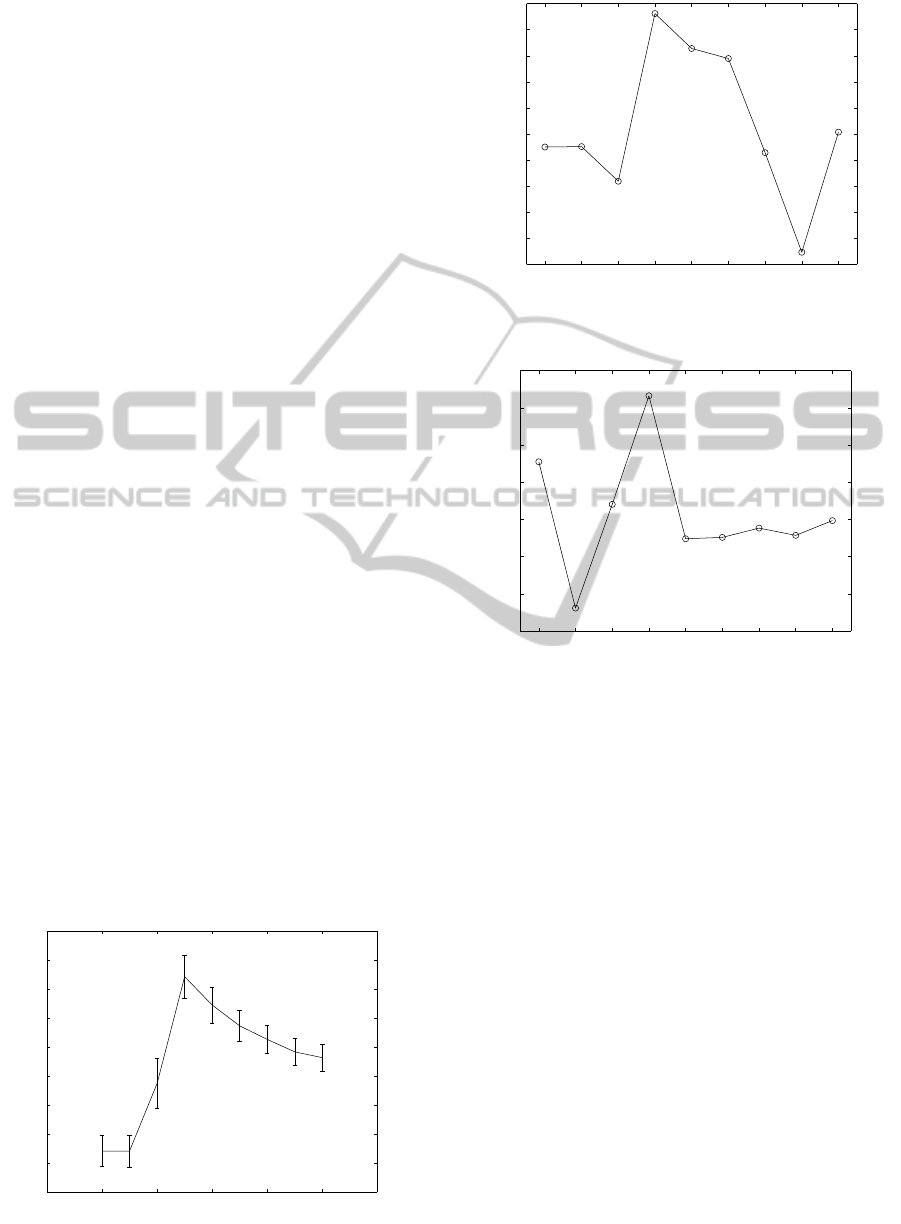
and 3 for standard HAC. Evolution of these statistics
as functionsof the numberof clusters, that can be seen
in Figures 6, 7 and 8, explain these results. Figure 6
shows the evolution of the Gap Statistic as a func-
tion of the number of clusters k for a realization of
the second data set. As can be seen, the criterion ini-
tially proposed gives k = 2. Figure 7 represents the
evolution of Centered Alignment Gap. The behavior
is rather erratic and explains the variations in the esti-
mated number of clusters. This can also be observed
for Weighted Delta Level Gap shown in Figure 8.
Furthermore, Delta Level Gap shows excellent
performances on data set 5, which cannot be classi-
fied using non kernel HAC while easily separated by
kernel HAC, as can be seen from Table 1.
According to all experiments we have done (not
all of them are presented here), we have observed that
the initial Gap Statistic of Tibshirani is not always
efficient in estimating the right number of clusters.
Looking for the maximum value instead of selecting
the value proposed as in equation 8, appears to be a
possible alternative. However, the Delta Level Gap
seems to be the most reliable estimate among those
we have studied and potentially one of the less sensi-
tive to the null distribution of the data.
0 2 4 6 8 10 12
0.4
0.5
0.6
0.7
0.8
0.9
1
1.1
1.2
1.3
Number of clusters k
Gap statistic
Figure 6: Number of clusters using Gap Statistic.
2 3 4 5 6 7 8 9 10
−0.02
−0.01
0
0.01
0.02
0.03
0.04
0.05
0.06
0.07
0.08
Number of clusters k
Centered Alignment Gap
Figure 7: Number of clusters using Centered Alignment
Gap.
2 3 4 5 6 7 8 9 10
−1.5
−1
−0.5
0
0.5
1
1.5
2
Number of clusters k
Weighted Delta Level Gap
Figure 8: Number of clusters using Weighted Delta Level
Gap.
5 CONCLUSIONS
In this paper,we have proposed Kernel HAC as a clus-
tering tool. It is robust for clustering separable classes
which have a small between-class dispersion in the
input space. Using an adequate Gap Statistic, it also
allows determination of the number of clusters in the
data. Out of them, simulation results have shown that
Delta Level Gap, one of our criteria, outperforms the
conventional Gap Statistic in many cases. Our future
work will focus on new methods for determining the
optimal kernel parameter. A few work has been done
which has already shown good prospects. Then, ker-
nel engineering (adaptation of the kernel function to
the data) will be considered.
REFERENCES
Aizerman, A., Braverman, E. M., and Rozoner, L. (1964).
Theoretical foundations of the potential function
KernelHierarchicalAgglomerativeClustering-ComparisonofDifferentGapStatisticstoEstimatetheNumberofClusters
261

method in pattern recognition learning. Automation
and remote control, 25:821–837.
Barbar´a, D. and Jajodia, S. (2002). Applications of data
mining in computer security, volume 6. Springer.
Bezdek, J. C., Ehrlich, R., and Full, W. (1984). Fcm: The
fuzzy c-means clustering algorithm. Computers &
Geosciences, 10(2):191–203.
Cali´nski, T. and Harabasz, J. (1974). A dendrite method for
cluster analysis. Communications in Statistics-theory
and Methods, 3(1):1–27.
Cortes, C. and Vapnik, V. (1995). Support-vector networks.
Machine learning, 20(3):273–297.
Driver, H. E. and Kroeber, A. L. (1932). Quantitative ex-
pression of cultural relationships. University of Cali-
fornia Press.
Filippone, M., Camastra, F., Masulli, F., and Rovetta, S.
(2008). A survey of kernel and spectral methods for
clustering. Pattern recognition, 41(1):176–190.
Fraley, C. and Raftery, A. E. (1998). How many clusters?
which clustering method? answers via model-based
cluster analysis. The computer journal, 41(8):578–
588.
Girolami, M. (2002). Mercer kernel-based clustering in fea-
ture space. Neural Networks, IEEE Transactions on,
13(3):780–784.
Gordon, A. D. (1996). Null models in cluster validation. In
From data to knowledge, pages 32–44. Springer.
Harman, H. H. (1960). Modern factor analysis.
Hartigan, J. A. (1975). Clustering Algorithms. John Wiley
& Sons, Inc., New York, NY, USA, 99th edition.
Kaufman, L. and Rousseeuw, P. J. (2009). Finding groups
in data: an introduction to cluster analysis, volume
344. Wiley-Interscience.
Kim, D.-W., Lee, K. Y., Lee, D., and Lee, K. H. (2005).
Evaluation of the performance of clustering algo-
rithms in kernel-induced feature space. Pattern
Recognition, 38(4):607–611.
Krzanowski, W. J. and Lai, Y. (1988). A criterion for deter-
mining the number of groups in a data set using sum-
of-squares clustering. Biometrics, pages 23–34.
Mac Queen, J. et al. (1967). Some methods for classifi-
cation and analysis of multivariate observations. In
Proceedings of the fifth Berkeley symposium on math-
ematical statistics and probability, volume 1, page 14.
California, USA.
Mercer, J. (1909). Functions of positive and negative type,
and their connection with the theory of integral equa-
tions. Philosophical transactions of the royal society
of London. Series A, containing papers of a mathe-
matical or physical character, 209:415–446.
Milligan, G. W. and Cooper, M. C. (1985). An examination
of procedures for determining the number of clusters
in a data set. Psychometrika, 50(2):159–179.
Muller, K.-R., Mika, S., Ratsch, G., Tsuda, K., and
Scholkopf, B. (2001). An introduction to kernel-based
learning algorithms. Neural Networks, IEEE Transac-
tions on, 12(2):181–201.
Murtagh, F. (1983). A survey of recent advances in hierar-
chical clustering algorithms. The Computer Journal,
26(4):354–359.
Olson, C. F. (1995). Parallel algorithms for hierarchical
clustering. Parallel computing, 21(8):1313–1325.
Pr´ıncipe, J. C., Liu, W., and Haykin, S. (2011). Kernel
Adaptive Filtering: A Comprehensive Introduction,
volume 57. John Wiley & Sons.
Qin, J., Lewis, D. P., and Noble, W. S. (2003). Kernel hi-
erarchical gene clustering from microarray expression
data. Bioinformatics, 19(16):2097–2104.
Sch¨olkopf, B., Smola, A., and M¨uller, K.-R. (1998). Non-
linear component analysis as a kernel eigenvalue prob-
lem. Neural computation, 10(5):1299–1319.
Shawe-Taylor, N. and Kandola, A. (2002). On kernel target
alignment. Advances in neural information processing
systems, 14:367.
Sneath, P. H., Sokal, R. R., et al. (1973). Numerical taxon-
omy. The principles and practice of numerical classi-
fication.
Sugar, C. A. and James, G. M. (2003). Finding the num-
ber of clusters in a dataset. Journal of the American
Statistical Association, 98(463).
Tibshirani, R., Walther, G., and Hastie, T. (2001). Estimat-
ing the number of clusters in a data set via the gap
statistic. Journal of the Royal Statistical Society: Se-
ries B (Statistical Methodology), 63(2):411–423.
Vapnik, V. (2000). The nature of statistical learning theory.
springer.
ICPRAM2014-InternationalConferenceonPatternRecognitionApplicationsandMethods
262
