
Fusion of Audio-visual Features using Hierarchical Classifier Systems for
the Recognition of Affective States and the State of Depression
Markus K¨achele, Michael Glodek, Dimitrij Zharkov, Sascha Meudt and Friedhelm Schwenker
Institute of Neural Information Processing, Ulm University, Ulm, Germany
Keywords:
Emotion Recognition, Multiple Classifier Systems, Affective Computing, Information Fusion.
Abstract:
Reliable prediction of affective states in real world scenarios is very challenging and a significant amount of
ongoing research is targeted towards improvement of existing systems. Major problems include the unrelia-
bility of labels, variations of the same affective states amongst different persons and in different modalities
as well as the presence of sensor noise in the signals. This work presents a framework for adaptive fusion of
input modalities incorporating variable degrees of certainty on different levels. Using a strategy that starts with
ensembles of weak learners, gradually, level by level, the discriminative power of the system is improved by
adaptively weighting favorable decisions, while concurrently dismissing unfavorable ones. For the final deci-
sion fusion the proposed system leverages a trained Kalman filter. Besides its ability to deal with missing and
uncertain values, in its nature, the Kalman filter is a time series predictor and thus a suitable choice to match
input signals to a reference time series in the form of ground truth labels. In the case of affect recognition, the
proposed system exhibits superior performance in comparison to competing systems on the analysed dataset.
1 INTRODUCTION
Estimation of the affective state and the subsequent
use of the gathered information is the main focus
of a novel subfield of computer science called affec-
tive computing. People’s affective states can be in-
ferred using many different modalities such as cues
for facial expression, speech analysis or biophysio-
logical measurements. Advances in affective comput-
ing in recent years have come from facial expression
recognition in laboratory-like environments (Kanade
et al., 2000), emotional speech recognition from acted
datasets (Burkhardt et al., 2005) and induced emo-
tions in biophysiological measurements to emotion
recognition from unconstrained audio visual record-
ings with non-acted content (Valstar et al., 2013)
or audio-visual data with biophysiological measure-
ments in human computer interaction scenarios. In
contrast to the first advances in affective computing,
the problems nowadays aim at nonacted and nonob-
strusive recordings. As a result, the difficulties in
classification have significantly increased.
Speech signals are appealing for emotion recog-
niton because they can be processed conveniently
and their analyses present promising ways for future
research (Fragopanagos and Taylor, 2005; Scherer
et al., 2003; Scherer et al., 2008).
One of the main issues in designing automatic
emotion recognition systems is the selection of the
features that can reflect the corresponding emotions.
In recent years, several different feature types proved
to be useful in the context of emotion recognition
from speech: Modulation Spectrum, Relative Spectral
Transform - Perceptual Linear Prediction (RASTA-
PLP), and perceived loudness features (Palm and
Schwenker, 2009; Schwenker et al., 2010), the Mel
Frequency Cepstral Coefficients (MFCC) (Lee et al.,
2004), or the Log Frequency Power Coefficients
(LFPC) (Nwe et al., 2003). Recently, Voice Quality
features havereceived increased attention, due to their
ability to represent different speech styles and thus are
directly applicable for emotion distinction (Lugger
and Yang, 2006; Luengo et al., 2010; Scherer et al.,
2012). Because there is still no consensus on which
features are best suited for the task, often many dif-
ferent features are computed and the decision which
ones to use is handed over to a fusion or feature selec-
tion stage.
Recognition of facial expressions has been a pop-
ular and very active field of research since the emer-
gence of consumer cameras and fast computing hard-
ware. Recent contributions advance the field in the di-
rections of recognition of action units (e.g. (Senechal
et al., 2012) using local Gabor binary pattern his-
671
Kächele M., Glodek M., Zharkov D., Meudt S. and Schwenker F..
Fusion of Audio-visual Features using Hierarchical Classifier Systems for the Recognition of Affective States and the State of Depression.
DOI: 10.5220/0004828606710678
In Proceedings of the 3rd International Conference on Pattern Recognition Applications and Methods (ICPRAM-2014), pages 671-678
ISBN: 978-989-758-018-5
Copyright
c
2014 SCITEPRESS (Science and Technology Publications, Lda.)

tograms and multikernel learning), acted emotions
(e.g. (Yang and Bhanu, 2011), introducing the emo-
tion avatar image) and spontaneous emotions (refer to
(Zeng et al., 2009) for an overview).
Besides solely relying on a single modality, classi-
fication systems can be improvedusing multiple input
channels. The task at hand is inherently bimodal and
thus using a system that combines results of the audio
and video channel is favorable. In the literature, mul-
tiple classifier systems that rely on information fusion
show superior results over single modality systems as
indicated by the results of the previous AVEC editions
(W¨ollmer et al., 2013) and works such as (Glodek
et al., 2012; Glodek et al., 2013) as well as the other
challenge entries (S´anchez-Lozano et al., 2013) and
(Meng et al., 2013), that also employ a multilayered
system to combine audio and video. Besides affect,
recognition of the state of depression has gained in-
creased attention in recent years especially with views
on advances in medicine and psychology. Automatic
recognition of the state of depression can be helpful
and is therefore a desirable goal, because plausible
estimations can be very difficult due to individual dis-
crepancies and often require substantial knowledge
and expertise and/or self-assessed depression rating
of the people themselves (Cohn et al., 2009).
The remainder of this work is organized as fol-
lows. In the next section, the dataset is introduced.
In Section 3 the audio and video approaches are pre-
sented together with the fusion approach for the final
layer of the recognition pipeline. Section 4 presents
results on the dataset and Section 5 closes the paper
with concluding remarks.
2 DATASET
The utilized dataset is a subset of the audio-visual
depressive language (AViD) corpus as used in the
2013 edition of the audio visual emotion challenge
(AVEC2013) (Valstar et al., 2013). The original set
consists of 292 subjects, each of whom was recorded
between one and four times. The recordings feature
people of both genders, spanning the range of ages be-
tween 18 and 63 (with a mean of 31.5 years). For the
recordings, the participants were positioned in front
of a laptop and were instructed to read, sing and tell
stories.
The dataset features two kinds of labels divided
into affect and depression. The affect labels consist
of the dimensions arousal and valence (Russell and
Mehrabian, 1977). Arousal is an indicator of the ac-
tivity of the nervous system. Valence is a measure for
the pleasantness of an emotion. The affect labels were
collected by manual annotation of the videos as a per
frame value for valence and arousal in the range of
[−1, 1].
The depression labels were self-assessed by the
participants using the Beck Depression Inventory-II
questionnaire. The label comprised a single depres-
sion score for a whole video sequence. The challenge
set consists of 150 recordings selected from the origi-
nal set and split into Training, Development and Test
subsets. It is important to notice, that several partic-
ipants appeared in more than one subset. The video
channel features 24-bit color video at a sampling rate
of 30 Hz at a resolution of 640×480. The audio chan-
nel was recorded using an off-the-shelf headset at a
sampling rate of 41 kHz. Both modalities are avail-
able for the recognition task. For more details, the
reader is referred to (Valstar et al., 2013).
3 METHODS
For the prediction of the states of affect and depres-
sion, different approaches are introduced for the sin-
gle modalities. The audio approach is based on a mul-
titude of different features, including voice quality
features, in combination with statistical analysis. A
novel forward/backward feature selection algorithm
is used to reduce the number of features to the most
discriminative ones. The video modality was handled
using a cascade of classifiers on multiple levels with
the intention to adaptively weigh the most significant
classification results of the preceeding level and thus
omitting interfering results. The final fusion step is
carried out using a trainable Kalman filter. The deci-
sion for two different approaches for the two modali-
ties was based on the characteristics of the data. The
video channel results in a very large amount of data
of the same type, where it is important to extract the
most significant instances, while the features for the
audio channel were modelled so that a very rich set
of different descriptors results in fewer, but more dis-
criminant instances.
3.1 Modified Forward Backward
Feature Selection for the Audio
Modality
Three groups of segmental feature types have been
extracted (spectral, voice quality and prosodic fea-
tures), containing nine feature families.
Spectral features have been computed on Ham-
ming windowed 25 ms frames with 10 ms overlap.
MFCC have been found to be useful in the task of
ICPRAM2014-InternationalConferenceonPatternRecognitionApplicationsandMethods
672

(derivative)
Figure 1: A single cycle of an example glottal flow (top)
and its derivative (bottom). t
l
, t
p
, and t
e
are different char-
acteristic values as defined in (Scherer et al., 2012). Image
adapted from (Scherer et al., 2012).
emotion classification (Lee et al., 2004). In (Nwe
et al., 2003) it is shown that Log Frequency Power
Coefficients (LFPC) even outperform MFCC.
Voice Quality features describe the properties of
the glottal source. By inverse filtering, the influence
of the vocal tract is compensated to a great content
(Lugger and Yang, 2007).
Spectral gradient parameters are estimated by us-
ing the fact that the glottal properties “open quo-
tient”, “glottal opening”, “skewness of glottal pulse”
and “rate of glottal closure” each affect the excita-
tion spectrum of the speech signal in a dedicated fre-
quency range and thus reflect the voice quality of the
speaker (Lugger and Yang, 2006).
The peak slope parameter as proposed in (Kane
and Gobl, 2013) is based on features derived from
wavelet based decomposition of the speech signal.
g(t) = −cos(2π f
n
t) ·exp(−
t
2
2τ
2
) (1)
Where f
n
=
f
s
2
and τ =
1
2f
n
. The decomposition of the
speech signal, x(t), is then achieved by convolving
it with g(
t
s
i
), where s
i
= 2
i
and i = 0, ..., 5. Finally,
a straight regression line is fitted to the peak ampli-
tudes obtained by the convolutions. The peak slope
parameter is the slope of this regression line.
The remaining voice quality features are calcu-
lated on the basis of the glottal source signal (Drug-
man et al., 2011). An example of a glottal flow and its
derivative is shown in Fig. 1. The following features
are calculated for each period of the glottal flow:
The normalized amplitude quotient (NAQ) (Airas
and Alku, 2007) is calculated using Eq. 2 where f
ac
and d
peak
are the amplitudes at the points t
p
and t
e
respectively and T is the duration of the glottal flow.
NAQ =
f
ac
d
peak
· T
(2)
The quasi-open quotient (QOQ) (Airas and Alku,
2007) is defined as the duration during which the glot-
tal flow is 50% above the minimum flow.
The Maxima Dispersion Quotient (MDQ) (Kane
and Gobl, 2013) is a parameter designed to quan-
tify the dispersion of the Maxima derived from the
wavelet decomposion of the glottal flow in relation to
the glottal closure instant (GCI).
The glottal harmonics (GH) are the first eight har-
monics of the glottal source spectrum.
Altogether, 79 segmental features are extracted.
Suprasegmental Features
Suprasegmental features represent long-term infor-
mation of speech. Therefore, an estimation of the
segmental features over a certain time period is made.
This period is defined as an utterance bound by two
consecutive pauses.
As in (Luengo et al., 2010), for every segmental
feature and its first and second derivatives, six statis-
tics (Mean, Variance, Minimum, Range, Skewness
and Kurtosis) were computed, leading to a 79× 3×
6 = 1422 dimensional feature set.
Feature Selection
In a first step, the forward-selection algorithm was ap-
plied to find the most promising features. Starting
with an empty feature set, in every iteration the algo-
rithm aims at increasing the classification accuracy by
adding the best feature to the current set in a greedy
fashion.
For termination, the long-term stopping criterion
introduced in (Meudt et al., 2013), was used. The
algorithm is terminated at timestep t, if no improve-
ment has been achieved during the last k time steps,
in comparison to the accuracy acc(t − (k + 1)). The
resulting feature set is then used as the initial feature
set for a backward elimination algorithm. Here, the
least promising features are eliminated from the set in
each iteration. The algorithm terminates if all but one
feature have been eliminated. The final feature set is
the one, which led to the highest accuracy during the
processing of the backward elimination algorithm.
3.2 Video
Face Detection and Extraction
The first step in the visual feature extraction pipeline
was robust detection and alignment of face im-
ages. Detection was done using the Viola and Jones’
boosted Haar cascade (Viola and Jones, 2001) fol-
lowed by landmark tracking using a constrained local
FusionofAudio-visualFeaturesusingHierarchicalClassifierSystemsfor
theRecognitionofAffectiveStatesandtheStateofDepression
673

model (Saragih et al., 2011) to keep record of salient
points over time. Based on those located keypoints,
an alignment procedure was carried out in order to
normalize the face position. Normalization is an es-
sential part in order to work with faces of different
people and sequences with a large amount of mo-
tion. A least-squares optimal affine transformation
was used to align selected points and based on the
found mapping, the image was interpolated to a fixed
reference frame.
Feature extraction
For the feature extraction stage, local appearance
descriptors in the form of local phase quantization
(LPQ) (Ojansivu and Heikkil, 2008) were used. The
LPQ descriptor was initially designed for blur insen-
sitive texture classification but in recent work it has
been shown, that it can be successfully applied to the
recognition of facial expressions (Jiang et al., 2011).
The idea behind LPQ is that the phase of a Fourier
transformed signal is invariant against blurring with
isotropic kernels (e.g. Gaussian). The first step is to
apply a short-time Fourier transform (STFT) over a
small neighbourhood N
x
to the image I.
STFT
u
u
u
{I(x
x
x)} = S(u
u
u, x
x
x) =
∑
y
y
y∈N
x
I(x
x
x− y
y
y)e
−i2πu
u
u
T
y
y
y
(3)
the vector u
u
u contains the desired frequency coef-
ficients. The Fourier transform is computed for the
four sets of coefficients: u
0
= [0, a]
T
, u
1
= [a, 0]
T
,
u
2
= [a, a]
T
, and u
3
= [a, −a]
T
with a being a small
frequency value depending on the blur characteristic.
The four Fourier coefficient pairs are stored in a vec-
tor q
q
q according to
q
q
q = [Re{S(u
u
u
i
, x
x
x)}, Im{S(u
u
u
i
, x
x
x)}]
T
, i = 0, . . . , 3 (4)
Since the coefficients of neighbouring pixels are
usually highly correlated, a whitening procedure is
carried out, followed by quantization based on the
sign of the coefficient:
q
lpq
i
=
1 if q
i
≥ 0
0 otherwise
The bitstring q
lpq
is then treated as an 8-bit decimal
number, which is the final coefficient for that pixel.
The face image is divided into subregions for which
individual 256-dimensional histograms are computed
by binning the LPQ coefficients. The feature vector
for every image is a concatenation of all the subregion
histograms.
LPQ descriptors were chosen because they
showed a superior performance over other descrip-
tors such as local binary patterns (LBP) (Ojala et al.,
1996).
Base Classification
The base of the video classification scheme consists
of an ensemble of sparse regressors, trained on a dif-
ferent subset of the training set. The algorithm of
choice was support vector regression (ε-SVR). The
dataset was preprocessed so that multiple neighbour-
ing frames were averaged using a binomial filter ker-
nel in order to minimize redundancein the dataset and
to shrink it to a more manageable size. The available
labels were also integrated using the filter kernel.
An ensemble of regressors is a suitable choice of
base classifiers, because training a single one would
on the one hand be difficult because of the sheer
amount of available data and on the other hand be-
cause of the datas nature: In emotion recognition,
classes are rarely linearly separable and a large over-
lap exists. A single classifier would thus either de-
grade because it learns contradicting data points with
uncertain labels or would create a “best fit”, that
means vaguely approximates the trend of the data.
Both cases are not desirable and due to that, several
regressors are trained on subsets of the data and com-
bined in a later step. The results of the regressor stage
are integrated by training a multilayer neural network
on the outputs with the real labels as training signal.
All experiments were conducted using a radial ba-
sis function kernel for the SVR with cross validation
applied to (a subset of) the Development set to deter-
mine the optimal parameter ranges.
Fusion Layer for Base Classifiers
The amount of available data allowed the training of
more than one regressor ensembles. Thus, the ar-
chitecture was enlarged horizontally by adding ad-
ditional ensembles and vertically by adding another
multilayer perceptron (MLP) to combine the outputs
of the second layer (with the first layer being a sin-
gle support vector regression node). In Figure 2, the
details of the architecture are illustrated.
3.3 Fusion
Modern fusion algorithms have to meet new require-
ments emerging in pattern recognition. Algorithms
start to shift towards real-time application which are
utilized on mobile devices with limited resources.
Furthermore, state-of-the-art approaches have to pro-
vide elaborated treatments to handle missing classi-
fier decisions which occur for instance due to sensor
failures (Glodek et al., 2012). In recent results, we
showed that the well-known Kalman filter (Kalman,
1960) can successfully be applied to perform classi-
fier fusion (Glodek et al., 2013). However, in this pa-
ICPRAM2014-InternationalConferenceonPatternRecognitionApplicationsandMethods
674
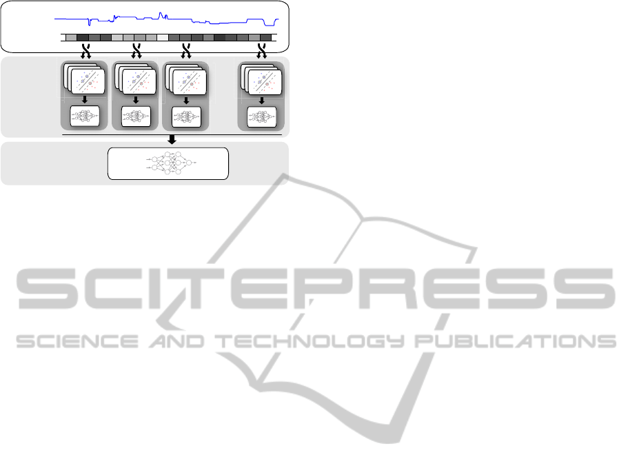
SVR
SVR
ensemble
. . .
. . .
Input
data
Fusion
layer
. . .
MLP
SVR
MLP
SVR
MLP
SVR
MLP
MLP
Figure 2: Illustration of the employed fusion scheme. Data
subsets are randomly chosen and deal as input for an ensem-
ble of support vector regressors. The results of the regres-
sion stage then act as input for a multilayer neural network
that is trained to combine the results based on the ground
truth label at that position. On top of the ensemble group is
another multilayer perceptron, that combines the intermedi-
ate outputs of the regressor ensemble stage.
per, the parameters of the model are determined using
the learning algorithm, rather than performing an ex-
haustive search in the parameter space.
The Kalman filter is driven by a temporal se-
quence of M classifier decisions X ∈ [0, 1]
M× T
where
T denotes the time. Each classifier decision is repre-
sented by a single value ranging between zero and one
which is indicating the class membership predicted
given a modality. The Kalman filter predicts the most
likely decision which might have produced the per-
ceived observation by additionally modeling the noise
and the probability of false decisions. Furthermore,
missing classifier decisions, e.g. due to sensor fail-
ures, are natively taken care of. The Kalman filter
infers the most likely classifier outcome given the pre-
ceding observations within two steps. First, the belief
state is derived by
bµ
t+1
= a · µ
t
+ b· u (5)
b
σ
t+1
= a · σ
t
· a + q
m
(6)
where in Equation 5, the predicted classifier decision
of the last time step and the control u is weighted lin-
early by the transition model a and the control-input
model b. The control u offers the option to have a bias
to which the prediction attracted to, e.g. in a two-class
problem with predictions ranging between [−1, 1] this
could be the least informative classifier combination:
0.0. However, the applied model presumes that the
mean of the current estimate is identical to the pre-
vious one such that the last term was omitted. The
covariance of the prediction is given by
b
σ
t
and ob-
tained by combining the a posteriori covariance with
a noise model q
m
to be derived for each modality. The
successive update step has to be performed for every
classifier m and makes use of the residuum γ, the in-
novation variance s and the Kalman gain k
t+1
:
γ = x
mt+1
− h·bµ
t+1
(7)
s = h·
b
σ
t+1
· h + r
m
(8)
k
t+1
= h·
b
σ
t+1
· s
−1
(9)
where h is the observation model mapping the pre-
dicted quantity to the new estimate and r
m
is the error
model, which is modeling the error of the given deci-
sions. The updated mean and variance are given by
µ
t+1
= bµ
t+1
+ k
t+1
· γ (10)
σ
t+1
=
b
σ
t
− k· s· k (11)
A missing classifier decision is replaced by a mea-
surement prior ˜x
mt
equal to 0.0 and a corresponding
observation noise ˜r
m
. In order to learn the noise and
error model, we make use of the standard learning al-
gorithm for Kalman filter (Bishop, 2006).
4 RESULTS
The performance of the proposed system is measured
in two ways as in the original challenge: For de-
pression recognition the error is measured in mean
absolute error (MAE) and root mean square error
(RMSE) averaged over all participants. In case of af-
fect recognition Pearson’s correlation coefficient av-
eraged over all participants is applied. The higher the
correlation value, the better the match between the es-
timation and the labels. A maximum correlation value
of 1.0 indicates perfect match, while a value of 0.0 in-
dicates no congruence. In order to be able to compare
the different methods, intermediate results are com-
puted for every channel as well as for the combined
system. A comparison with the baseline system (Val-
star et al., 2013) and with competing architectures is
given.
Prediction of the State of Depression
For the recognition of the state of depression, the re-
sults for the single modalities as well as a fusion ap-
proach can be found in Table 1. Since the videos were
labeled with a single depression score per file, the pre-
dictions of the individual modalities were averaged
to a single decision (for audio) or to about 30 − 60
depending on the length of the file (for video). The
best performance is achieved by the video modality.
For both, the Development and Test set, the video
modality outperformed the baseline results. The au-
dio modality outperforms the baseline only on the not
publicly available challenge Test partition. The fu-
sion was conducted by training an MLP (3 neurons,
FusionofAudio-visualFeaturesusingHierarchicalClassifierSystemsfor
theRecognitionofAffectiveStatesandtheStateofDepression
675

Table 1: Results for depression recognition. Performance
is measured in mean absolute error (MAE) and root mean
square error (RMSE) over all participants.
Development
Approach Modality MAE RMSE
Baseline Audio 8.66 10.75
Baseline Video 8.74 10.72
(Meng et al., 2013) Fusion 6.94 8.56
Proposed Audio 9.35 11.40
Proposed Video 7.03 8.82
Proposed Fusion 8.30 9.94
Test
Approach Modality MAE RMSE
Baseline Audio 10.35 14.12
Baseline Video 10.88 13.61
Proposed Audio 9.47 11.48
Proposed Video 8.97 10.82
Proposed Fusion 9.09 11.19
(Meng et al., 2013) Fusion 8.72 10.96
1 hidden layer) on the Development set with audio
and video scores as input and the original label as
training signal. Because of the large performance gap
between audio and video, the fusion did not result
in better performance in comparison to the modali-
ties on their own. The work by (Meng et al., 2013)
focuses solely on depression recognition and com-
prises different feature extraction mechanisms com-
bines with motion history histograms (MHH) for time
coding for both video and audio, followed by a partial
least squares regressor for each modality and a com-
bination using a weighted sum rule. The comparison
between the proposed system and the one by Meng
et al. indicates similar performance on the Test set.
Their system seems to yield a closer fit in the sense
of MAE, but system proposed here offers a smaller
RMSE, which indicates that there are less points that
have a high deviation from the true label (which is
penalized quadratically using this error measure).
Prediction of the State of Affect
For the audio modality, the predictions were made
on a per-utterance basis and then interpolated to the
number of video frames for the respective video. The
video modality again shows superior performance
overthe audio modality. The multilevelarchitecture is
able to deal with the shear amount of data and is able
to favor the meaningful samples while letting mean-
ingless ones vanish in the depth of the architecture.
The system can be seen as a cascade of filters. The
filter created by each layer has to deal with more ab-
stract data
1
. The recently proposed deep learning ar-
1
The raw input is only available for the first layer while
each other layer has to deal with nonlinear combinations
and abstractions created on lower layers.
chitectures (Hinton et al., 2006) share some similari-
ties, however, while a deep belief net is usually com-
posed of many layers with a high number of simple
neurons, the nodes of the proposed architecture are
complex classifiers and the information propagation
takes place only in one direction
2
. The base ensem-
ble of the utilized system contains seven support vec-
tor regressors. Each of them was trained on 15% of
the training set, aggregated in subsets using bagging.
The fusion network was an MLP with 20 neurons in a
single hidden layer with a sigmoid transfer function.
The second layer consisted of five of those ensembles,
combined using an MLP with 30 neurons in the hid-
den layer.
The combination of the video and the audio
modality using the Kalman filter seems very promis-
ing: In almost every case, the fusion of audio and
video exhibits the best performance over all the sin-
gle modalities. The results can be found in Table 2. In
Figure 3, the resulting trajectories using the Kalman
filter are shown.
The architecture proposed by (S´anchez-Lozano
et al., 2013) is somewhat similar to the proposed sys-
tem in that there are also fusion stages that combine
intermediate results on different levels. Their system
leverages an early-fusion type combination for differ-
ent feature sets (LBP and Gabor for video and various
features like MFCC, energy, and statistical moments
for audio), followed by fusion of the two modalities.
The final fusion step is a correlation based fusion us-
ing both arousal and valence estimations as input.
In comparison, the performance of the proposed
system is unmatched by any of the other approaches
on the Test set. On the Development set, the per-
formance of the baseline system is superior to every
other approach, however it heavily drops on the Test
set. Overfitting on the Development set could be an
explanation for this circumstance.
5 CONCLUSIONS
In this work, a recognition system for psychological
states such as affect or the state of depression has been
presented. Various methods of information fusion (ei-
ther in a hierarchy of classifiers or as means for final
decision fusion) are used to extract salient informa-
tion from the datastreams. For the recognition of de-
pression, the proposed system outperforms the base-
line and is comparable to competing systems while
for the state of affect, the results are superior to any
2
While a deep belief net uses multiple forward and back-
ward passes through the net, here only the forward passes
are used to train subsequent layers.
ICPRAM2014-InternationalConferenceonPatternRecognitionApplicationsandMethods
676
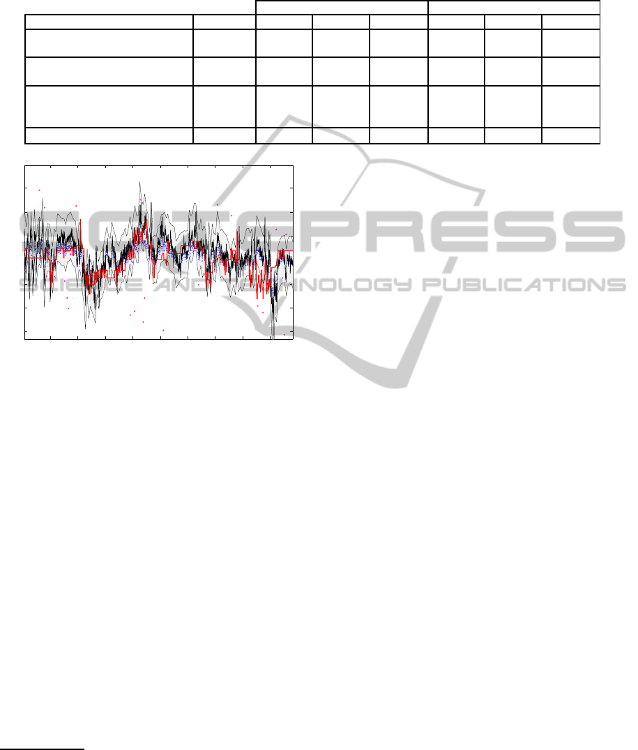
Table 2: Results for affect recognition. The baseline system performs very well on the Development set, however much worse
on the Test set. This might be caused by overfitting. An improvement over each individual modality is reached (in most cases)
using the Kalman filter for the final fusion step. The proposed system is able to outperform the system by (S´anchez-Lozano
et al., 2013) on the Test set.
Development Test
Approach Modality Valence Arousal Average Valence Arousal Average
Baseline Audio 0.338 0.257 0.298 0.089 0.090 0.089
Baseline Video 0.337 0.157 0.247 0.076 0.134 0.105
(S´anchez-Lozano et al., 2013) A+V 0.173 0.154 0.163 n.a. n.a. n.a.
(S´anchez-Lozano et al., 2013) Fusion 0.167 0.192 0.180 0.135 0.132 0.134
Proposed Audio 0.094 0.103 0.099 0.107 0.114 0.111
Proposed Video 0.153 0.098 0.126 0.118 0.142 0.130
Proposed Fusion 0.134 0.156 0.145 0.150 0.170 0.160
AVEC 2013 winner
3
Fusion 0.141
time
valence
-0.6
-0.4
-0.2
0
0.2
0.4
0.6
Figure 3: Kalman filter fusion of the modalities for one ran-
domly selected participant. Input of the video modality in
blue dots, inputs of the audio modality in magenta. The
ground truth is given in red while black is the final estima-
tion µ. The gray corridor around the estimation corresponds
to σ, a certainty value of the estimation. As can be seen, the
trajectory of the label is matched to a high degree.
of the discussed approaches on the Test set (includ-
ing the challenge winner). The proposed system can
be extended in different directions. For example, the
early fusion of audio and video could be promising as
well as investigating deeper architectures of complex
classifiers and/or the use of deep belief networks as
base classifiers. The overall relatively low correlation
values of all approaches indicate that the problem is
far from being solved and much more research has to
be dedicated to feature extraction, classification meth-
ods and fusion mechanisms.
REFERENCES
Airas, M. and Alku, P. (2007). Comparison of multiple
voice source parameters in different phonation types.
3
See http://sspnet.eu/avec2013/ for details. (Meng et al.,
2013) is listed as the winner. The paper however, does not
contain results for the affect subchallenge. (Checked on 07.
January, 2014)
In INTERSPEECH, pages 1410–1413.
Bishop, C. M. (2006). Pattern Recognition and Machine
Learning. Springer.
Burkhardt, F., Paeschke, A., Rolfes, M., Sendlmeier, W.,
and Weiss, B. (2005). A database of German emo-
tional speech. In Proceedings of Interspeech 2005,
pages 1517–1520.
Cohn, J., Kruez, T., Matthews, I., Yang, Y., Nguyen, M. H.,
Padilla, M., Zhou, F., and De la Torre, F. (2009).
Detecting depression from facial actions and vocal
prosody. In Affective Computing and Intelligent In-
teraction and Workshops (ACII 2009)., pages 1–7.
Drugman, T., Bozkurt, B., and Dutoit, T. (2011). Causal–
anticausal decomposition of speech using complex
cepstrum for glottal source estimation. Speech Com-
munication, 53(6):855–866.
Fragopanagos, N. and Taylor, J. (2005). Emotion recogni-
tion in human-computer interaction. Neural Networks,
18:389–405.
Glodek, M., Reuter, S., Schels, M., Dietmayer, K., and
Schwenker, F. (2013). Kalman filter based classifier
fusion for affective state recognition. In Proceedings
of the International Workshop on Multiple Classifier
Systems (MCS), volume 7872 of LNCS, pages 85–94.
Springer.
Glodek, M., Schels, M., Palm, G., and Schwenker, F.
(2012). Multi-modal fusion based on classification us-
ing rejection option and Markov fusion networks. In
Proceedings of the International Conference on Pat-
tern Recognition (ICPR), pages 1084–1087. IEEE.
Hinton, G. E., Osindero, S., and Teh, Y.-W. (2006). A fast
learning algorithm for deep belief nets. Neural Com-
put., 18(7):1527–1554.
Jiang, B., Valstar, M. F., and Pantic, M. (2011). Action
unit detection using sparse appearance descriptors in
space-time video volumes. In Proceedings of IEEE
International Conference on Automatic Face and Ges-
ture Recognition, pages 314–321. IEEE.
Kalman, R. E. (1960). A new approach to linear filtering
and prediction problems. Transactions of the ASME
— Journal of Basic Engineering, 82(Series D):35–45.
Kanade, T., Cohn, J., and Tian, Y. (2000). Comprehensive
database for facial expression analysis. In Automatic
Face and Gesture Recognition, 2000., pages 46–53.
FusionofAudio-visualFeaturesusingHierarchicalClassifierSystemsfor
theRecognitionofAffectiveStatesandtheStateofDepression
677

Kane, J. and Gobl, C. (2013). Wavelet maxima disper-
sion for breathy to tense voice discrimination. Audio,
Speech, and Language Processing, IEEE Transactions
on, 21(6):1170–1179.
Lee, C. M., Yildirim, S., Bulut, M., Kazemzadeh, A.,
Busso, C., Deng, Z., Lee, S., and Narayanan, S. S.
(2004). Emotion recognition based on phoneme
classes. In Proceedings of ICSLP 2004.
Luengo, I., Navas, E., and Hern´aez, I. (2010). Feature anal-
ysis and evaluation for automatic emotion identifica-
tion in speech. Multimedia, IEEE Transactions on,
12(6):490–501.
Lugger, M. and Yang, B. (2006). Classification of different
speaking groups by means of voice quality parame-
ters. ITG-Fachbericht-Sprachkommunikation 2006.
Lugger, M. and Yang, B. (2007). The relevance of
voice quality features in speaker independent emotion
recognition. In Acoustics, Speech and Signal Process-
ing, 2007. ICASSP 2007. IEEE International Confer-
ence on, volume 4, pages IV–17. IEEE.
Meng, H., Huang, D., Wang, H., Yang, H., AI-Shuraifi, M.,
and Wang, Y. (2013). Depression recognition based
on dynamic facial and vocal expression features us-
ing partial least square regression. In Proceedings of
AVEC 2013, AVEC ’13, pages 21–30. ACM.
Meudt, S., Zharkov, D., K¨achele, M., and Schwenker, F.
(2013). Multi classifier systems and forward back-
ward feature selection algorithms to classify emo-
tional coloured speech. In Proceedings of the Inter-
national Conference on Multimodal Interaction (ICMI
2013).
Nwe, T. L., Foo, S. W., and De Silva, L. C. (2003). Speech
emotion recognition using hidden markov models.
Speech communication, 41(4):603–623.
Ojala, T., Pietikinen, M., and Harwood, D. (1996). A com-
parative study of texture measures with classification
based on featured distributions. Pattern Recognition,
29(1):51 – 59.
Ojansivu, V. and Heikkil, J. (2008). Blur insensitive tex-
ture classification using local phase quantization. In
Elmoataz, A., Lezoray, O., Nouboud, F., and Mam-
mass, D., editors, Image and Signal Processing, vol-
ume 5099 of LNCS, pages 236–243. Springer Berlin
Heidelberg.
Palm, G. and Schwenker, F. (2009). Sensor-fusion in neu-
ral networks. In Shahbazian, E., Rogova, G., and
DeWeert, M. J., editors, Harbour Protection Through
Data Fusion Technologies, pages 299–306. Springer.
Russell, J. A. and Mehrabian, A. (1977). Evidence for a
three-factor theory of emotions. Journal of Research
in Personality, 11(3):273 – 294.
S´anchez-Lozano, E., Lopez-Otero, P., Docio-Fernandez, L.,
Argones-R´ua, E., and Alba-Castro, J. L. (2013). Au-
diovisual three-level fusion for continuous estimation
of russell’s emotion circumplex. In Proceedings of
AVEC 2013, AVEC ’13, pages 31–40. ACM.
Saragih, J. M., Lucey, S., and Cohn, J. F. (2011). De-
formable model fitting by regularized landmark mean-
shift. Int. J. Comput. Vision, 91(2):200–215.
Scherer, K. R., Johnstone, T., and Klasmeyer, G. (2003).
Handbook of Affective Sciences - Vocal expression of
emotion, chapter 23, pages 433–456. Affective Sci-
ence. Oxford University Press.
Scherer, S., Kane, J., Gobl, C., and Schwenker, F. (2012).
Investigating fuzzy-input fuzzy-output support vector
machines for robust voice quality classification. Com-
puter Speech and Language, 27(1):263–287.
Scherer, S., Schwenker, F., and Palm, G. (2008). Emotion
recognition from speech using multi-classifier sys-
tems and rbf-ensembles. In Speech, Audio, Image and
Biomedical Signal Processing using Neural Networks,
pages 49–70. Springer Berlin Heidelberg.
Schwenker, F., Scherer, S., Schmidt, M., Schels, M., and
Glodek, M. (2010). Multiple classifier systems for the
recognition of human emotions. In Gayar, N. E., Kit-
tler, J., and Roli, F., editors, Proceedings of the 9th In-
ternational Workshop on Multiple Classifier Systems
(MCS’10), LNCS 5997, pages 315–324. Springer.
Senechal, T., Rapp, V., Salam, H., Seguier, R., Bailly, K.,
and Prevost, L. (2012). Facial action recognition com-
bining heterogeneous features via multikernel learn-
ing. Systems, Man, and Cybernetics, Part B: Cyber-
netics, IEEE Transactions on, 42(4):993–1005.
Valstar, M., Schuller, B., Smith, K., Eyben, F., Jiang, B.,
Bilakhia, S., Schnieder, S., Cowie, R., and Pantic,
M. (2013). Avec 2013: The continuous audio/visual
emotion and depression recognition challenge. In
Proceedings of AVEC 2013, AVEC ’13, pages 3–10.
ACM.
Viola, P. and Jones, M. (2001). Rapid object detection using
a boosted cascade of simple features. In Computer Vi-
sion and Pattern Recognition, 2001. CVPR 2001. Pro-
ceedings of the 2001 IEEE Computer Society Confer-
ence on, volume 1, pages I–511–I–518 vol.1.
W¨ollmer, M., Kaiser, M., Eyben, F., Schuller, B., and
Rigoll, G. (2013). LSTM-modeling of continuous
emotions in an audiovisual affect recognition frame-
work. Image and Vision Computing, 31(2):153 – 163.
Affect Analysis In Continuous Input.
Yang, S. and Bhanu, B. (2011). Facial expression recogni-
tion using emotion avatar image. In Automatic Face
Gesture Recognition and Workshops (FG 2011), 2011
IEEE International Conference on, pages 866–871.
Zeng, Z., Pantic, M., Roisman, G. I., and Huang, T. S.
(2009). A survey of affect recognition methods: Au-
dio, visual, and spontaneous expressions. pages 39–
58.
ICPRAM2014-InternationalConferenceonPatternRecognitionApplicationsandMethods
678
