Hierarchical Energy-transfer Features

Radovan Fusek, Eduard Sojka, Karel Mozd

n and Milan

Surkala

Technical University of Ostrava, FEECS, Department of Computer Science

17. listopadu 15, 708 33 Ostrava-Poruba, Czech Republic

Keywords:

Object Detection, Recognition, SVM, Image Descriptors, Feature Selection.

Abstract:

In the paper, we propose the novel and efﬁcient object descriptors that are designed to describe the appearance

of the objects. The descriptors are called as Hierarchical Energy-Transfer Features (HETF). The main idea

behind HETF is that the shape of the objects can be described by the function of energy distribution. In the

image, the transfer of energy is solved by making use of physical laws. The function of the energy distribution

is obtained by sampling, after the energy transfer process; the image is divided into the cells of variable sizes

and the values of the function is investigated inside each cell. The proposed descriptors achieved very good

detection results compared with the state-of-the-art methods (e.g. Haar, HOG, LBP features). We show the

robustness of the descriptors for solving the face detection problem.

1 INTRODUCTION

The area of computer vision includes many tasks that

have been well researched in recent years. In this pa-

per, we will focus on the problem of object descrip-

tion and detection. It is clear that the images con-

tain many objects of interest. The goal of the ob-

ject detection systems is to ﬁnd the location of these

objects in the images (e.g. cars, faces, pedestrians).

For example, the vehicle detection systems are cru-

cial for trafﬁc analysis or intelligent scheduling, the

people detection systems can be useful for automo-

tive safety, and the face detection systems are the key

part of face recognition systems. Typically, the detec-

tion algorithms are composed from two main parts in

the area of feature-based detectors. The extraction of

image features is the ﬁrst part. The second part is cre-

ated by the trainable classiﬁers that handle the ﬁnal

classiﬁcation (object/non-object). In this paper, our

contribution will be focused on the ﬁrst part; on the

extraction of image features.

The proposed features are based on the idea that

the appearance of objects can be described by the

function of the distribution of energy; if we speak

about the energy transfer in this paper, we have the

transfer of heat in mind. We suppose that the im-

age is a rectangular plate with the thermal conduc-

tivity properties; big gradients represent the low con-

ductivity and vice versa. In the process of obtain-

ing the proposed features, the temperature sources

are placed into the image. The transfer of tempera-

ture starts from the sources at the same time and the

transfer is carried out during a chosen time. The dis-

tribution of temperature is investigated after the tem-

perature transfer. The vector of features that is com-

posed of this distribution is then used as an input for

the SVM classiﬁer. In essence, the proposed features

are slightly inspired by HOG but instead of the his-

tograms of oriented gradients we investigate the dis-

tributions of temperature. In this paper, we show the

properties of the proposed features for solving the

problem of face detection and we show that using the

function of temperature distribution, the faces can be

described with a reasonable number of features with

good detection results. The preliminary version of the

presented method (without the hierarchical improve-

ment) was used for face detection in (Fusek et al.,

2013).

The paper is organized as follows. In Section 2,

we present an overview of the state-of-the-art feature-

based detectors. In Section 3, we describe the extrac-

tion of the proposed features in detail, and we show

the experiments and results in Section 4.

2 RELATED WORKS

In this section, we will especially focus on the im-

age features that are extracted over the sliding win-

dow that are divided into the dense areas (due to the

fact that the proposed descriptors are also calculated

695

Fusek R., Sojka E., Mozd

n K. and Šurkala M..

Hierarchical Energy-transfer Features.

DOI: 10.5220/0004829506950702

In Proceedings of the 3rd International Conference on Pattern Recognition Applications and Methods (ICPRAM-2014), pages 695-702

ISBN: 978-989-758-018-5

 2014 SCITEPRESS (Science and Technology Publications, Lda.)

within the dense regular blocks).

In recent years, the object detectors that are based

on the edge analysis providing the valuable informa-

tion about the objects of interest have been used in

many detection tasks. In this area, the Histograms of

Oriented Gradients (HOG) (Dalal and Triggs, 2005)

are considered as the state-of-the-art method. In

essence, the HOG descriptors can be regarded as a

dense version of the SIFT features. In HOG, a sliding

window is used for recognition. The window is di-

vided into small connected cells in the process of ob-

taining HOG descriptors. The histograms of gradients

are calculated for each cell. It is desirable to normal-

ize the histograms across a large block of image. As a

result, a vector of values is computed for each position

of window. This vector is then used for recognition,

e.g. by the Support Vector Machine (SVM) classiﬁer

(Boser et al., 1992). Many methods and applications

that are based on HOG have been successfully pre-

sented in recent years. The PHOG descriptors that use

the pyramid image representation were presented in

(Bosch et al., 2007). The classical HOG-based detec-

tor was used for detecting upper bodies for automated

upper body pose estimation in (Ferrari et al., 2008).

Felzenszwalb et al. (Felzenszwalb et al., 2010) pro-

posed the part-based detector that is based on HOG.

In this method, the objects are represented using mix-

tures of deformable HOG part models and these mod-

els are trained using a discriminative method.

Haar-based descriptors represent the next possi-

bility for object description. The main idea behind

the Haar-like features is that the features can encode

the differences in mean intensities between two rect-

angular areas. For instance, in the problem of face

detection, the regions around the eyes are lighter than

the areas of the eyes; the regions below or on top

the eyes have different intensities that the eyes it-

self. These speciﬁc characteristics can be simple en-

coded by one two-rectangular feature, and the value

of this feature can be calculated as the difference be-

tween the sum of the pixels inside the two rectangles.

The Haar-like features which are similar to Haar ba-

sis function have ﬁrst been proposed by Papageor-

giou and Poggio (Papageorgiou and Poggio, 2000).

In their paper, the Haar-like features are combined

with the SVM classiﬁer. The authors used the three

types of Haar features (vertical, horizontal, diagonal)

that were able to encode the changes in the intensi-

ties at various locations, scales, and orientations. The

authors also reported promising performance in the

tasks of face, car, and people detection in their paper.

Since then, the Haar-like features and their modiﬁca-

tions have been used in many works. The paper of

Viola and Jones (Viola and Jones, 2001) contributed

to the popularity of Haar-like features. They pro-

posed the object detection framework based on the

image representation called the integral image com-

bined with the rectangular features, and AdaBoost al-

gorithm (Freund and Schapire, 1995). The extension

of the Haar feature set has been presented by Lienhart

et al.(Lienhart and Maydt, 2002). In this paper, the

authors presented 45

◦

rotated features that are able to

reduce the false alarm and achieve more accurate face

detection.

Local Binary Patterns (LBP) that were introduced

by Ojala et al.(Ojala et al., 1996) for texture analy-

sis can also be used for object description. The main

idea behind LBP is that the local image structures (so

called micro patterns such as lines, edges, spots, and

ﬂat areas) around each pixel can be efﬁciently en-

coded by comparing every pixel with its neighboring

pixels; in the basic form, every pixel is compared with

its neighbors in the 3 × 3 region. The result of the

comparison is the 8-bit binary number for each pixel;

in the 8-bit binary number, the value 1 means that the

value of center pixel is greater than the neighbor and

vice versa. The histogram of these binary numbers

is then used to encode the appearance of the region.

The important properties of LBP are resistance to

lighting changes and low computational complexity.

Duo to their properties, LBP have been used in many

recognition tasks, especially for facial image analy-

sis. In (Hadid et al., 2004), LBP were used for solving

the face detection problem in low-resolution images.

Multi-block Local Binary Patterns (MB-LBP) for face

detection were proposed in (Zhang et al., 2007). The

paper of Tan and Triggs (Tan and Triggs, 2010) pro-

posed the face recognition method using robust pre-

processing based on the Difference of Gaussian image

ﬁlter combined with LBP in which the binary LBP

code is replaced by the ternary LTP code.

In the next section, we will show the process of

extraction of the proposed features.

3 HIERARCHICAL

ENERGY-TRANSFER

FEATURES

As was mentioned before, the main idea behind the

proposed features is based on the fact that the ap-

pearance of objects can be efﬁciently described by the

function of temperature distribution in the following

way.

Suppose the theoretical image that contains one

object (with one area), and suppose that this object

has very thin edges; theoretically, the edges can be

ICPRAM2014-InternationalConferenceonPatternRecognitionApplicationsandMethods

696

inﬁnitely thin (the gradient of brightness of this theo-

retical image is shown in the second row in Fig. 1).

Suppose that this object of interest (with the very thin

edges) is analyzed by the functions of gradient sizes

and directions. The meaningful sample values of this

function can be difﬁcult to obtain; it is difﬁcult to ob-

tain (by the samples) the information about the thin

edges (it may happen that the samples will not hit the

thin edges). On the other hand, the function of tem-

perature distribution does not make problems during

sampling. Suppose that the source of constant temper-

ature is placed inside the considered object; say that

into the gravity center of object (Fig. 1(a)). Inside the

image, the temperature transfer (from this source) can

be solved by making use of physical laws. It means

that the gradients of the object can be considered as

the thermal insulator; high gradients indicate the low

conductivity and vice versa. After the temperature

transfer that is carried out during a chosen time, the

area of this object will contain a certain distribution

of temperature (Fig. 1(b)), and the function of tem-

perature distribution inside this object can be investi-

gated. In this function, the areas with approximately

constant temperature values are important and it is an

easy matter to hit them by samples.

under the rectangular basin

inside the object

temperature

t = 0

t > 0

(a)

(b)

Figure 1: The image with one object and one source of tem-

perature. The value of temperature is depicted by the inten-

sity of red color.

Finally, the temperature distribution reﬂects the

presence of objects and their parts and the appearance

of object of interest can be described by the distribu-

tion (with a relatively small amount of descriptors),

which is the main idea of the method we propose.

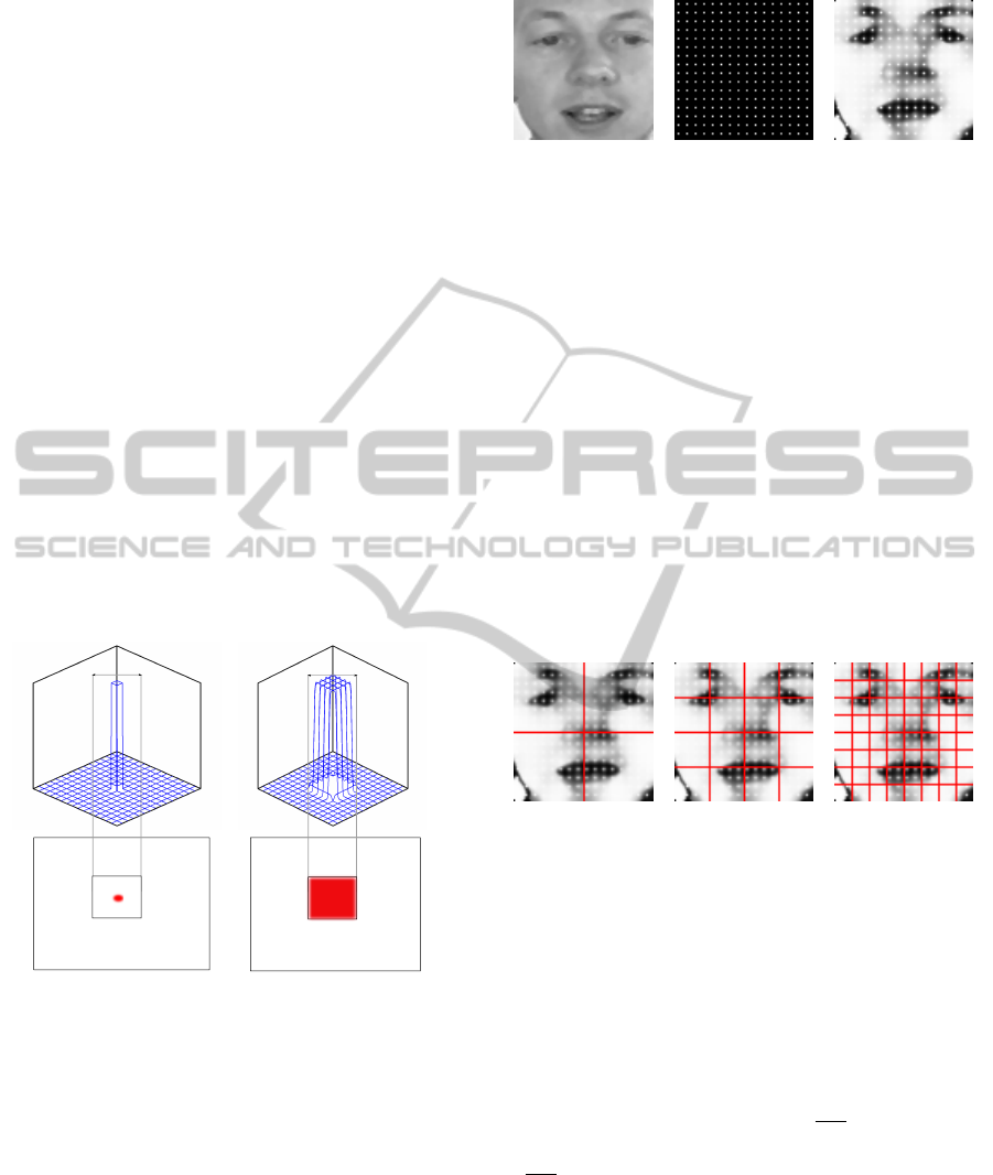
It is clear that the real images consist of objects

with different areas (Fig. 2(a)) and one temperature

source will not be enough to cover all areas. There-

fore, we chose the location of temperature sources in

the form of regular grid (Fig. 2(b)). At the time t = 0,

(a) (b) (c)

Figure 2: The real-life image (a). The regular grid of

sources (b). The visualization of distribution of temperature

from these sources (c). The value of temperature is depicted

by the level of brightness.

the temperature of constant value 1.0 is attached to the

source locations; other places inside the image have

zero temperature at the time t = 0. The temperature

transfer that starts from all sources at the same time is

carried out during a chosen time t. Once the temper-

ature transfer inside the image is obtained, the func-

tion of temperature distribution inside the image is in-

vestigated (the example of temperature distribution is

shown in Fig. 2(c)). For this purpose, the image is

iteratively divided into the ﬁner spatial cells; i.e. we

recursively divide the image into the cells of varying

size (Fig. 3). In general, the image at hierarchical

level l has 4

cells. Inside each cell, the distribution is

investigated.

l = 1 l = 2 l = 3

Figure 3: The different hierarchical levels of the cells.

Let I(x, y, t) be the function of temperature (at lo-

cation (x, y) and the time t) that is determined. We

can compute the mean temperature in every cell; Iµ

stands for the mean temperature of the i-th cell at the

time t. We use the mean cell temperatures as the val-

ues in the feature vector. For the additional informa-

tion and for the precise description of the temperature

distribution, we use the histogram of the temperature

distribution that is also determined inside the cells.

Each cell is represented by the

|M| + Iµ

dimen-

sion vector, where |M| is the size of the cell, and

|M| represents the number of histogram bins; the

ﬁnal vector of features is composed of the mean tem-

perature and from the histograms of each cell at each

hierarchical level. For example, for one cell of size

400 pixels (20 × 20), we compute the 20 histogram

bins and the mean temperature of the cell Iµ

, and the

feature vector of this cell is the vector with dimension

d = 21. The process of composing the ﬁnal feature

HierarchicalEnergy-transferFeatures

697

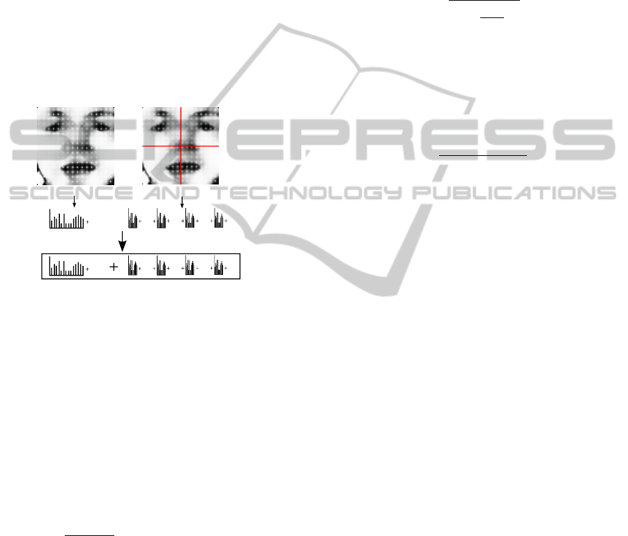
vector for the levels l = 0 and l = 1 is shown in Fig.

In the detection phase, we use the sliding window

technique. The size of detection window is set to the

size of training samples. Once the temperature ﬁeld

inside the whole input image is computed, the detec-

tion window scans this ﬁeld and the feature vector

is composed inside the window. The vector is then

used as an input for the SVM classiﬁer. It is impor-

tant to mention that the classical HOG descriptors are

not rotationally invariant. Since the proposed descrip-

tors are similar to the HOG descriptors (in the sense

that the features are computed in a grid in both ap-

proaches), this limitation also occurs in the proposed

descriptors. Similarly as in HOG, the scale invariance

is achieved by rescaling the images.

Final feature vector

l = 1

l = 0

Figure 4: The process of composing the ﬁnal feature vector.

In the case that the image has size 80 ×80 pixels, the vector

dimension is d = 81 at the level l = 0 (80 bin histogram +

mean temperature Iµ

). The level l = 1 contains 4 cells with

size 40 × 40; the 40 bin histogram with the mean tempera-

ture Iµ

is calculated in each cell (41 values for each cell)

and the vector dimension is d = 164. In this case, the ﬁnal

feature vector is composed as the sum of vector at the level

l = 0 and l = 1.

For the practical realization of the method, it is

important to mention that the thermal ﬁeld inside the

image can be solved by making use of the following

equation (Perona and Malik, 1990)

∂I(x, y, t)

∂t

= div(c∇I), (1)

where I represents the temperature at a position (x, y)

and at a time t, div is a divergence operator, ∇I is the

temperature gradient and c stands for thermal con-

ductivity. For the source points and arbitrary time

t ∈ [0, ∞), we set I(x

, y

, t) = 1, where (x

, y

) are the

coordinates of the source points (i.e. we hold the tem-

perature constant during the whole process of trans-

fer, which is in contrast with the usual diffusion ap-

proaches). In all remaining points, we take into ac-

count the initial condition I(x, y, 0) = 0. We solve the

equation iteratively. The conductivity in Eq. 1 is de-

termined by

c = g(

), (2)

where E is an edge estimate. We deﬁne the edge es-

timate E as the gradient of original image E = ∇B,

where B is the brightness function. The function g(·)

has the form of (Perona and Malik, 1990)

∇B

) =

1 +



∇B



, (3)

where K is a constant representing the sensitivity to

the edges (Perona and Malik, 1990). Once the tem-

perature ﬁeld over the input image is obtained (at a

chosen time t), the mean cell temperature Iµ

can be

obtained by making use of the formula

Iµ

I(x, y, t)dxdy

|M|

, (4)

where M stands for the cell area, and |M| is its size.

The Support Vector Machine classiﬁer with the radial

basis function kernel is trained over the proposed de-

scriptors in the next step to create the ﬁnal classiﬁer.

4 EXPERIMENTS

For the training phase, the positive set consists

of 2300 faces and 4300 non-faces. We used the

face images from the BIOID database (https://

www.bioid.com/downloads/software/bioid-face-

database.html) combined with the Extended Yale

Face Database B (Lee et al., 2005). We manually

cropped these images on the area of faces only.

The negative set consists of 3000 images that were

obtained from the MIT-CBCL database (http:/

/cbcl.mit.edu/software-datasets/FaceData2.html)

combined with the 1300 hard negative examples.

The training images (for the proposed method) were

resized to the size of 80×80 pixels. The visualization

of temperature distribution of faces is shown in Fig.

As we said before, we use the sliding window

technique in the detection phase. The size of detec-

tion window is set to 80 × 80 pixels (the size of train-

ing samples). We use the ﬁxed size of window that

scan the image in 12 different resolutions of input

image. The thermal ﬁeld is computed for each res-

olution. The example of visualization of temperature

function inside the whole input image (of one reso-

lution of input image) with the positive detections is

shown in Fig. 6.

ICPRAM2014-InternationalConferenceonPatternRecognitionApplicationsandMethods

698

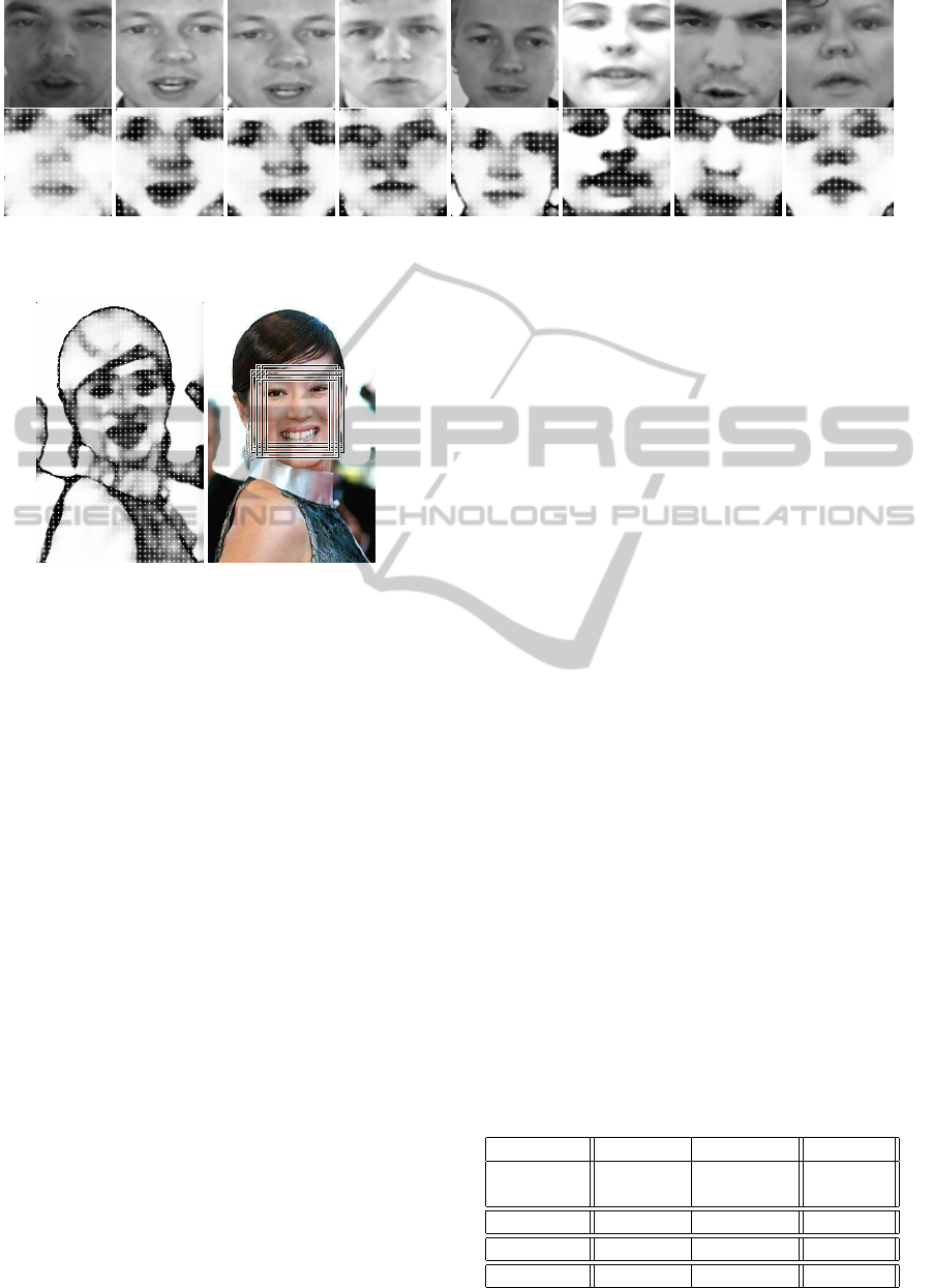
Figure 5: The visualization of distribution of temperature. The value of temperature is depicted by the level of brightness.

The ﬁrs row represents the original face images. The second row represents the visualization of temperature distribution.

Figure 6: The example of visualization of the temperature

ﬁeld. The left image shows the temperature function inside

the whole input image (the value of temperature is depicted

by the level of brightness). The right image shows the detec-

tion results without the postprocessing (the detection results

are not merged).

We experimented with the proposed method and

we suggest the following conﬁguration. The conﬁg-

uration of hierarchical energy transfer features is de-

noted as HET F. The size of temperature sources is 1

pixel and the distance between the sources is 5 pixels.

The time for temperature transfer is 250; this num-

ber represents the number of iterations because we

solve equation Eq. 1 iteratively. The mean tempera-

ture is computed inside each cell at levels 0, 1, 2, 3, 4;

it means that the mean temperature is computed in-

side the 341 cells (341 values in the feature vector).

Additionally to that, the histogram of the temperature

distribution is computed at levels 0, 1, 2, 3 (1200 val-

ues in the feature vector). Due to the fact that the cells

at l = 4 are relatively small (5× 5 pixels), we describe

these cells with the mean temperature only. Finally,

the ﬁnal feature vector consists of 1541 descriptors

for one position of sliding window; we experimented

with the different settings of levels and this conﬁgura-

tion achieved the best detection results. This conﬁg-

uration is also used for the visualization of proposed

features in Fig. 2, 3, 4, 5, and 6.

For comparison, we used the detectors that are

based on the HOG features, LBP (Local Binary Pat-

terns) features (Liao et al., 2007) and Haar features

(Viola-Jones detection framework).

For the HOG features we used the identical train-

ing sets like for the proposed features (2300 posi-

tive and 4300 negative samples) and we also used the

identical size of the samples (80×80pixels). We used

the typical parameters of HOG descriptors; the size

of block = 16 × 16 pixels; the size of cell = 8 × 8

pixels; the horizontal step size = 8 pixels; the num-

ber of bins = 9. This conﬁguration consists of 2916

HOG descriptors for one position of sliding window;

this conﬁguration is denoted as HOG. The Support

Vector Machine classiﬁer with Radial basis function

kernel is trained over the HOG descriptors create the

ﬁnal classiﬁer (similarly in the proposed descriptors).

For the detector based on the Viola-Jones detec-

tion framework and for the LBP-based detector, we

also used the identical training sets like for the pro-

posed features (2300 positive and 4300 negative sam-

ples) and we resized the training images to the size of

19 ×19. The detector based on the Viola-Jones detec-

tion framework is denoted as Haar, the detector based

on the LBP features is denoted as LBP. It is impor-

tant to mention that for these features, we created the

cascade classiﬁers.

To calculate the performance of approaches, we

collected the set of 200 images that contains 250 faces

from the Faces in the Wild dataset (Berg et al., 2005).

Before the process of performance calculation, the

positive detections were merged to one if at least 3

positive detections hit approximately one place in the

image. In Table 1, the detection results are shown.

The HOG-based detector achieved the good num-

Table 1: The detection performance.

Precision Sensitivity F1 score

HET F 98.15% 86.18% 91.77%

HET F

PCA

93.15% 93.90% 93.52%

HOG 68.75% 97.58% 80.67%

Haar 85.77% 87.55% 86.65%

LBP 62.96% 69.39% 66.02%

HierarchicalEnergy-transferFeatures

699

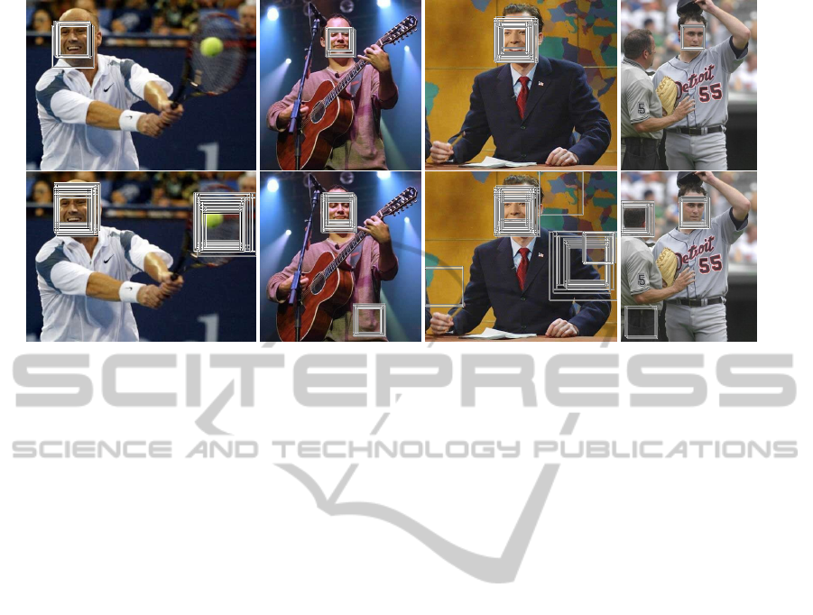
Figure 7: The differences between detection results. The ﬁrst row: the results of HET F. The second row: the results of HOG.

The results are without the postprocessing (the detection results are not merged).

ber of true positive detections (sensitivity 97.58%),

nevertheless, the number of false positives is larger

(precision 68.75%). For example, the spherical-like

objects (e.g. balls, tennis rackets) are the problem

for the HOG-based detector. In general, this detector

detected a lot of objects in the images and many of

these objects are not faces. In contrast, the proposed

method achieved the very promising numbers of true

positive detections (sensitivity 86.18%) and the pro-

posed descriptors also achieved the small number of

false positive detections (precision 98.15%) using 2×

less descriptors than in the HOG-based detector. We

experimented with the different settings of HOG de-

scriptors, however, without the increasing the datasets

for training, the HOG-based detector was not able to

achieve better results. The examples of the cases in

which the HOG-based detector failed are shown in

Fig. 7.

The cascade classiﬁer of Haar features achieved

better detection results than HOG descriptors (F1

score 86.65%). Nevertheless, this detector needed to

increase the number of training samples to achieved

better results. This problem also occurs in the LBP-

based detector (F1 score 66.02%).

With respect to the fact that the proposed features

had a low number of false positive detections (50

false positive detection windows of 7 million detec-

tion windows) and the number of descriptors (1541)

achieved the good results (F1 score 91.77%), we re-

duced the number of descriptors using PCA (Princi-

pal Component Analysis). To determine the number

of principal components, we used the 200 principal

components (corresponding to the largest eigenval-

ues); the ﬁnal feature vector is the vector with di-

mensionality d = 200. The detector that are based

on this subset of the proposed features is denoted as

HET F

PCA

The detector based on the subset of the proposed

features, achieved F1 score 93.52%; we note that the

number of false positives is larger sing this subset nev-

ertheless the detector achieved the best detection re-

sults (the examples in which the HET F

PCA

detector

failed are shown in 8). The detector also shows that

the appearance of the faces can be successfully de-

scribed using the distribution of temperature with a

relatively small set of the training samples and with a

relatively small set of descriptors compared with the

state-of-the-art descriptors. The detection results of

the detector based on the HET F

PCA

conﬁguration are

shown in Fig. 9.

If we discuss about the computational time of the

algorithm, the measurement of the time can be di-

vided into two parts. The ﬁrst part contains the time

that is necessary for the temperature transfer inside

the image. Since we solve the diffusion equation it-

eratively, the number of iterations has a major im-

pact on the computational time of this part. We have

developed the GPU (CUDA) and CPU (SSE/AVX)

versions for solving the temperature transfer process.

The computational time of GPU version is 40 mil-

liseconds, the time of CPU version is 150 millisec-

onds for 150 iterations and for the size of input image

640×480 pixels.

The second part contains the time that is required

for composing the feature vector. The mean tempera-

ture inside the rectangular cells is computed in a con-

stant time using the integral image. The calculation

of histogram of each cell took 1 millisecond for one

position of sliding window (80×80 pixels). Finally,

the recognition time of feature vector depends on the

ICPRAM2014-InternationalConferenceonPatternRecognitionApplicationsandMethods

700

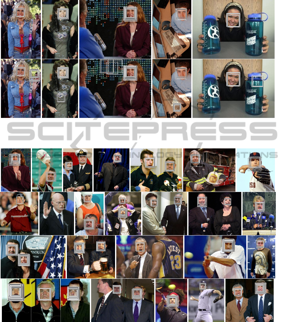
Figure 8: The detection results of HET F

PCA

in which the detector failed. The ﬁrst row: the results of HET F (without PCA).

The second row: the results of HET F

PCA

(with PCA). The results are without the postprocessing (the detection results are not

merged).

Figure 9: The detection results of HET F

PCA

. The results are without the postprocessing (the detection results are not merged).

chosen classiﬁer.

5 CONCLUSIONS

In the paper, we proposed the interesting method for

object description. The method is based on the fact

that the appearance of the objects can be described us-

ing the function of temperature distribution. The key

part of the proposed method is the process of tem-

perature transfer that is carried out during a chosen

time inside the image. This process is the most time-

consuming part of the method and we will focus on

the time complexity of the method in the future works.

HierarchicalEnergy-transferFeatures

701

However, compared with the state-of-the-art descrip-

tors, the proposed descriptors achieved the very good

detection results and we will also focus on detection

of other objects of interest using this method.

ACKNOWLEDGMENTS

This work was supported by the SGS in VSB Techni-

cal University of Ostrava, Czech Republic, under the

grant No. SP2014/170.

REFERENCES

Berg, T. L., Berg, A. C., Edwards, J., and Forsyth, D.

(2005). Who’s in the picture. In Saul, L. K., Weiss,

Y., and Bottou, L., editors, Advances in Neural Infor-

mation Processing Systems 17, pages 137–144. MIT

Press, Cambridge, MA.

Bosch, A., Zisserman, A., and Munoz, X. (2007). Repre-

senting shape with a spatial pyramid kernel. In Pro-

ceedings of the 6th ACM international conference on

Image and video retrieval, CIVR ’07, pages 401–408,

New York, NY, USA. ACM.

Boser, B. E., Guyon, I. M., and Vapnik, V. N. (1992).

A training algorithm for optimal margin classiﬁers.

In Proceedings of the 5th Annual ACM Workshop

on Computational Learning Theory, pages 144–152.

ACM Press.

Dalal, N. and Triggs, B. (2005). Histograms of oriented gra-

dients for human detection. In Computer Vision and

Pattern Recognition, 2005. CVPR 2005. IEEE Com-

puter Society Conference on, volume 1, pages 886 –

893 vol. 1.

Felzenszwalb, P., Girshick, R., McAllester, D., and Ra-

manan, D. (2010). Object detection with discrim-

inatively trained part-based models. Pattern Analy-

sis and Machine Intelligence, IEEE Transactions on,

32(9):1627–1645.

Ferrari, V., Marin-Jimenez, M., and Zisserman, A. (2008).

Progressive search space reduction for human pose es-

timation. In Computer Vision and Pattern Recogni-

tion, 2008. CVPR 2008. IEEE Conference on, pages

1–8.

Freund, Y. and Schapire, R. E. (1995). A decision-theoretic

generalization of on-line learning and an application

to boosting. In Proceedings of the Second Euro-

pean Conference on Computational Learning The-

ory, EuroCOLT ’95, pages 23–37, London, UK, UK.

Springer-Verlag.

Fusek, R., Sojka, E., Mozdren, K., and Surkala, M. (2013).

Energy-transfer features and their application in the

task of face detection. In Advanced Video and Signal

Based Surveillance (AVSS), 2013 10th IEEE Interna-

tional Conference on, pages 147–152.

Hadid, A., Pietikainen, M., and Ahonen, T. (2004). A dis-

criminative feature space for detecting and recogniz-

ing faces. In Computer Vision and Pattern Recogni-

tion, 2004. CVPR 2004. Proceedings of the 2004 IEEE

Computer Society Conference on, volume 2, pages II–

797–II–804 Vol.2.

Lee, K., Ho, J., and Kriegman, D. (2005). Acquiring linear

subspaces for face recognition under variable light-

ing. IEEE Trans. Pattern Anal. Mach. Intelligence,

27(5):684–698.

Liao, S., Zhu, X., Lei, Z., Zhang, L., and Li, S. Z. (2007).

Learning multi-scale block local binary patterns for

face recognition. In ICB, pages 828–837.

Lienhart, R. and Maydt, J. (2002). An extended set of haar-

like features for rapid object detection. In Image Pro-

cessing. 2002. Proceedings. 2002 International Con-

ference on, volume 1, pages I–900–I–903 vol.1.

Ojala, T., Pietik

ainen, M., and Harwood, D. (1996). A com-

parative study of texture measures with classiﬁcation

based on featured distributions. Pattern Recognition,

29(1):51–59.

Papageorgiou, C. and Poggio, T. (2000). A trainable system

for object detection. Int. J. Comput. Vision, 38(1):15–

33.

Perona, P. and Malik, J. (1990). Scale-space and edge detec-

tion using anisotropic diffusion. IEEE Trans. Pattern

Anal. Mach. Intell., 12:629–639.

Tan, X. and Triggs, B. (2010). Enhanced local texture fea-

ture sets for face recognition under difﬁcult lighting

conditions. Image Processing, IEEE Transactions on,

19(6):1635–1650.

Viola, P. and Jones, M. (2001). Rapid object detection using

a boosted cascade of simple features. In Computer Vi-

sion and Pattern Recognition, 2001. CVPR 2001. Pro-

ceedings of the 2001 IEEE Computer Society Confer-

ence on, volume 1, pages I–511 – I–518 vol.1.

Zhang, L., Chu, R., Xiang, S., Liao, S., and Li, S. Z. (2007).

Face detection based on multi-block lbp representa-

tion. In Proceedings of the 2007 international confer-

ence on Advances in Biometrics, ICB’07, pages 11–

18, Berlin, Heidelberg. Springer-Verlag.

ICPRAM2014-InternationalConferenceonPatternRecognitionApplicationsandMethods

702