Removing Motion Blur using Natural Image Statistics

Johannes Herwig, Timm Linder and Josef Pauli

Intelligent Systems Group, University of Duisburg-Essen, Bismarckstr. 90, 47057 Duisburg, Germany

Keywords:

Deconvolution, Bayesian Inference, Sparse Gradient Priors, Two-color Model, Parameter Learning.

Abstract:

We tackle deconvolution of motion blur in hand-held consumer photography with a Bayesian framework com-

bining sparse gradient and color priors for regularization. We develop a closed-form optimization utilizing

iterated re-weighted least squares (IRLS) with a Gaussian approximation of the regularization priors. The

model parameters of the priors can be learned from a set of natural images which resemble common image

statistics. We throughly evaluate and discuss the effect of different regularization factors and make sugges-

tions for reasonable values. Both gradient and color priors are current state-of-the-art. In natural images the

magnitude of gradients resembles a kurtotic hyper-Laplacian distribution, and the two-color model exploits

the observation that locally any color is a linear approximation between some primary and secondary col-

ors. Our contribution is integrating both priors into a single optimization framework and providing a more

detailed derivation of their optimization functions. Our re-implementation reveals different model parameters

than previously published, and the effectiveness of the color priors alone are explicitly examined. Finally, we

propose a context-adaptive parameterization of the regularization factors in order to avoid over-smoothing the

deconvolution result within highly textured areas.

1 INTRODUCTION

Removing motion blur due to camera shake is a spe-

cial branch of the ill-posed deconvolution problem.

Its speciﬁc challenges are the relatively large blur ker-

nels and image noise which usually is stronger here,

because camera shake is often caused by longer expo-

sure times during low-light photography where sensor

noise is inherently ampliﬁed due to higher analog gain

and shot noise. Another characteristic property is that

the blur kernels are not isotropic as with out-of-focus

blur, but instead these point spread functions (PSFs)

model the path of motion that a handheld camera un-

dertakes during the exposure time of the photograph,

and therefore the PSFs have a ridge-like and sparse

appearance (Liu et al., 2008).

We here tackle the problem of non-blind decon-

volution where the motion blur kernel (or PSF) is ex-

actly known a priori. In the real world, the gyroscope

of a mobile phone camera might give a good estimate

of the blur kernel. It is however not straightforward

to synchronize the gyroscope with start and end time

of the exposure. If motion information is not avail-

able at all, then we talk about blind deconvolution

where the blur kernel needs to be estimated solely

with the help of the blurred image at hand (Shi et al.,

2013; Dong et al., 2012a). Since this is rather difﬁcult

there are also some image fusion approaches, known

as semi-blind deconvolution (Yuan et al., 2007; Ito

et al., 2013; Wang et al., 2012). Thereby, multi-

ple differently blurred or otherwise multimodal im-

ages are taken from the same scene with the same or

different sensor which helps further constraining the

blur kernel (Yuan et al., 2007; Ito et al., 2013; Wang

et al., 2012). Our approach assumes a globally con-

stant blur kernel (Schmidt et al., 2013), but in gen-

eral image blur is space-varying (Sorel and Sroubek,

2012; Ji and Wang, 2012; Whyte et al., 2012; Gupta

et al., 2010) because objects at different distances in

the scene are blurred differently. Also, there are nat-

ural design constraints on the camera optics, so that

an image is usually sharper in the center compared to

its border. Additionally, there could be moving ob-

jects in the scene which overlay the movement of a

hand-held camera (Cho et al., 2012). However, usu-

ally only static scenes are considered when there is

only one image available.

1.1 Regularization

Most non-blind deconvolution approaches apply a

regularization term to the gradients of the image, by

125

Herwig J., Linder T. and Pauli J..

Removing Motion Blur using Natural Image Statistics.

DOI: 10.5220/0004830201250136

In Proceedings of the 3rd International Conference on Pattern Recognition Applications and Methods (ICPRAM-2014), pages 125-136

ISBN: 978-989-758-018-5

 2014 SCITEPRESS (Science and Technology Publications, Lda.)

−0.2−0.1 0 0.1 0.2

p(d

)

0 0.1 0.2 0.3 0.4 0.5

−5

ln p(|d

(a) Ground truth images

−0.2−0.1 0 0.1 0.2

p(d

)

0 0.1 0.2 0.3 0.4 0.5

−5

ln p(|d

(b) Blur added – typical camera shake blur

−0.2−0.1 0 0.1 0.2

p(d

)

0 0.1 0.2 0.3 0.4 0.5

−5

ln p(|d

−0.2−0.1 0 0.1 0.2

p(d

)

0 0.1 0.2 0.3 0.4 0.5

−5

ln p(|d

(d) Noise added (no blur!) – σ = 5%

Figure 1: Histograms of x-derivatives and x-derivative magnitudes. Colors correspond to Fig. 4.

penalizing steep gradients that could be indicative of

noise. Regularization based upon the `

norm (Gaus-

sian prior) and the `

norm (Laplacian prior, total

variation (Chan and Shen, 2005)) tend to oversmooth

the deconvolution results. The so-called sparse pri-

ors (Levin and Weiss, 2007; Levin et al., 2007b;

Li et al., 2013) more adequately capture the ob-

served hyper-Laplacian gradient distributions (Srivas-

tava et al., 2003; Huang, 2000). Here, the color

model-based regularization (Joshi et al., 2009) mo-

tivated by (Cecchi et al., 2010) imposes a two-color

model upon locally smooth regions. Thereby, we

concurrently make use of global and local sparseness

(Dong et al., 2012b) alike by using gradient and color

priors, respectively.

1.2 Sparse Gradient Prior

Most ’real’ images resemble a common gradient dis-

tribution (Levin and Weiss, 2007; Levin et al., 2007b;

Simoncelli, 1997). Under for example the `

-norm,

the gradient magnitude for a pixel i is calculated by

k(∇I)

∑

k=1

k,i

|, (1)

where d

k,i

represents the k-th partial derivative,

evaluated at pixel i of image I. Such a directional

derivative

:= vec(I ∗ G

) can be determined by

convolving the image I with derivative ﬁlter kernels

, like



1 −1



and



1 −1



and the second-

order derivatives

∂I

∂x

∂I

∂y

∂I

∂xy

In Fig. 1, we examine the gradient distributions of

the images from Fig. 4 and compare them with un-

wanted deconvolution results. These histogram plots

show that only the ground truth photographs exhibit

the kurtotic hyper-Laplacian shape, but blurry and

noisy images show totally different statistics. How-

ever, if the blur is linear and orthogonal to the direc-

tion of the derivative, then edges stay mostly intact –

but still the kurtotic tail is lowered (compare Fig. 1(a)

and 1(c)). Similarly to our analysis (Lin et al., 2011)

shows gradient distributions of examplarily patches of

motion blurred vs. sharp textures.

Instead of using gradients as a sparse prior, one

could use any kind of ﬁltering result that provides a

sparse representation of the image. We also tried the

learned ﬁlters approach within the Fields-of-Experts

(FoE) framework. Thereby we modiﬁed the MAT-

LAB code of (Weiss and Freeman, 2007) so that we

obtained a kurtotic curve model. Then we learned two

different sets of 5 and 25 ﬁlters of 15 × 15 pixels. As

opposed to (Schmidt et al., 2011) we did not ﬁnd an

increase in performance, but our results were compa-

rable to the sparse gradient prior.

1.3 Two-color Model

As in (Joshi et al., 2009), for each pixel ~c

of a latent

image estimate I, we deﬁne a pixel neighborhood –

e. g. using a square 5 × 5 window – and determine

the primary and secondary colors within this neigh-

borhood. Thereby, an initial two-color model is ob-

tained by k-means clustering (with k = 2). While k-

means provides a good heuristic for ﬁnding an ini-

tial two-color model, the drawback is that one color

sample can always only be assigned to exactly one

cluster, and therefore noise is not appropriately han-

ICPRAM2014-InternationalConferenceonPatternRecognitionApplicationsandMethods

126

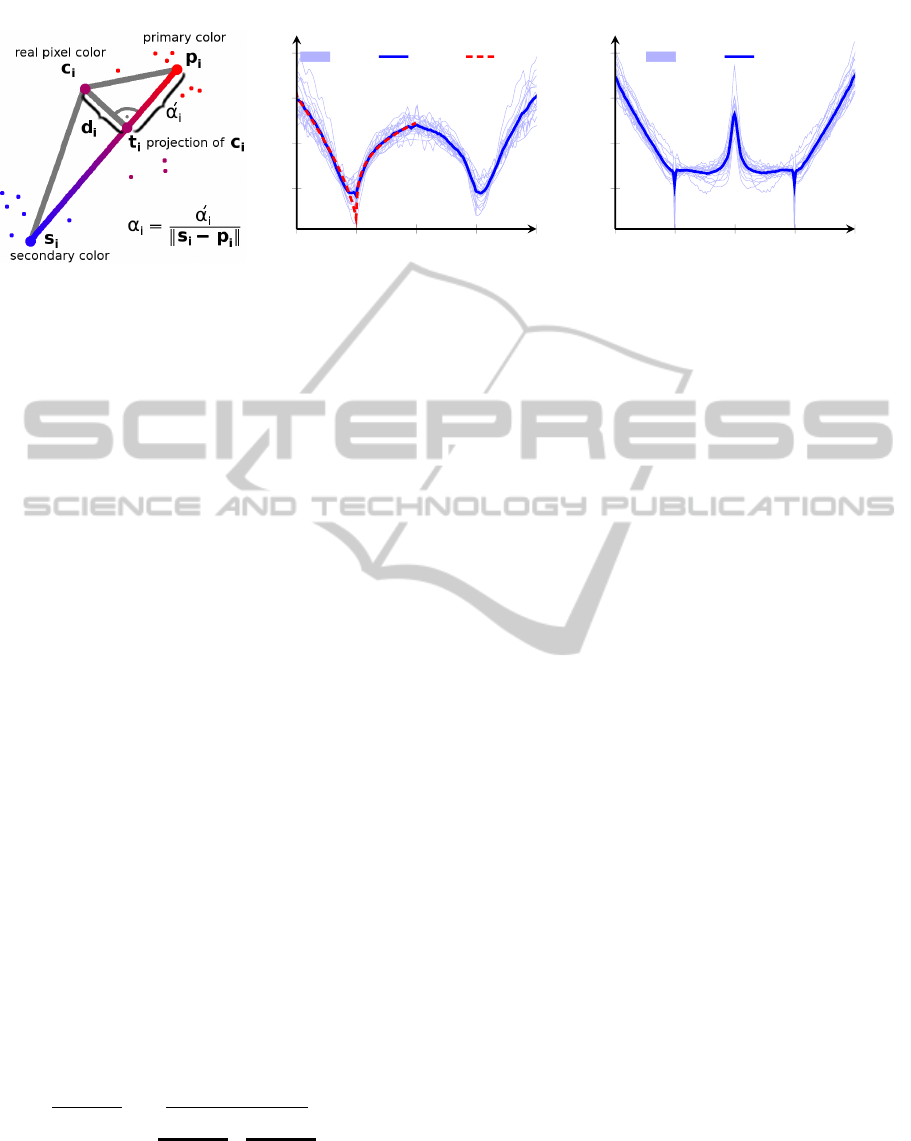
(a) Two-color model by Joshi

−0.5 0 0.5 1 1.5

− ln p(α)

data mean ﬁt

(b) α distribution after EM clustering

−0.5 0 0.5 1 1.5

− ln p(α)

data mean

Figure 2: The two-color model, and the accompanying alpha distributions learned from real images.

dled. A fuzzy expectation-maximization (EM) algo-

rithm based upon the method described in (Joshi et al.,

2009) therefore reﬁnes the color clusters. Finally, the

primary color ~p

is assigned to the cluster whose cen-

ter lies closest to the color of the center pixel ~c

deﬁn-

ing the neighborhood. The secondary color

is as-

signed to the other cluster. The two-color model as

depicted in Fig. 2(a) now works upon the assump-

tion that the color ~c

can be represented by a linear

interpolation between its associated primary and sec-

ondary colors ~p

∈ R

and

∈ R

, where α

∈ R is the

interpolation or mixing parameter (Joshi et al., 2009,

see eq. 7):

:= α

+ (1 − α

)~p

. (2)

In contrast to (Joshi et al., 2009), ~p

and

have been

swapped with regard to α

, such that α

is minimal at

instead of

, because this will simplify our IRLS

optimization later on.

2 THE COLOR PRIOR

The so-called alpha prior introduced by (Joshi et al.,

2009) penalizes α

values which would put the esti-

mated color ~c

far away from either the primary or

secondary color. The penalty is based upon the ob-

served α

distribution in natural images. The value of

for a pixel ~c

, given ~p

and

, is calculated using

(Joshi et al., 2009, eq. 10):

− ~p



(

− ~p

)

(

− ~p

)

(

− ~p

)



| {z }

∈R

(~c

− ~p

(3)

Typical distributions of α values determined from

natural images using either the reﬁned EM or bare k-

means color clustering are shown in Fig. 2(b) and

2(c). As in Fig. 2(b), these negative log-likelihoods

can be ﬁt with a piecewise hyper-Laplacian prior term

of the form

b|α

= b |

−

. (4)

We calculated the two-color model from about

400 images of the Berkeley image segmentation

database. For a custom set of ﬁt parameters, the

constructed color models were exported into Matlab

and approximate probability densities have been esti-

mated for each image using a Parzen window method.

Then, a non-linear least-squares ﬁt was performed us-

ing Matlab’s fminsearch() method for the piece-

wise hyper-Laplacian function described above. In

(Joshi et al., 2009) a 2 pieces ﬁt is proposed, but we

found that it is not sufﬁciently accurate for approach-

ing the statistics of the relatively noise-free ground

truth images. The resulting parameters for our 3

pieces ﬁt are:

a = 0.7153, b = 0.8066 for α

< −0.5;

a = 0.6448, b = 4.5318 for − 0.5 ≤ α

< 0;

a = 0.2298, b = 2.7372 for 0 ≤ α

2.1 Optimization Techniques

For weighted least squares (WLS) (Faraway, 2002,

p. 62), a weighting matrix W ∈ R

s×s

is introduced.

The WLS objective function therefore is

∑

k,l

= k~y − T~xk

= (~y − T~x)

W (~y − T~x),

(5)

where k · k

is the Mahalanobis distance when W =

−1

. In order to minimize this function, we need to

determine the gradient and set it equal to zero. The

WLS derivative

RemovingMotionBlurusingNaturalImageStatistics

127

∂

∂~x

k~y − T~xk

= −2T

W~y + 2T

W T~x (6)

yields the system of the so-called normal equations of

WLS (Gentle, 2007, p. 338)

W T )

| {z }

~x − T

W~y

| {z }

0 (7)

which represents a linear equation system of the form

A~x −

δ =

0. Here, A = T

W T is too large to be in-

verted in-place, and hence we use the CG (Conjugate

Gradient) method.

The M-estimator (Meer, 2004, p. 47) applies a ro-

bust penalty or loss function ρ to the error residuals

. For ρ(r

) := |r

, p 6= 2, the optimization becomes

non-linear. However, the iteratively re-weighted least

squares (IRLS) method (Scales et al., 1988; Scales

and Gersztenkorn, 1988) approximates the solution

by turning the problem into a series of WLS sub-

problems. A faster version of this algorithm for the

problem at hand is discussed in (Krishnan and Fergus,

2009). In each IRLS iteration, a new set of weights is

learned from the previous solution. For the ﬁrst it-

eration, all weights can be initialized with a constant

value. The weights w

of the diagonal WLS weighting

matrix W are ([1]: (Meer, 2004, p. 48); [2]: (Scales

et al., 1988, p. 332)):

(τ+1)

= w(r

(τ)

)

[1]

(τ)

dρ(r

(τ)

)

(τ)

[2]

= p|r

(τ)

p−2

. (8)

2.2 Minimizing the Alpha Prior

As already shown in Fig. 2(b), the α

distribution is

bimodal since both α

= 0 and α

= 1 are minima and

the distribution is symmetric at α

= 0.5. However,

since we want to bias the observed color ~c

to the pri-

mary color ~p

at α

= 0, only the unimodal prior (rep-

resented by the red, dashed line) is used. The weights

of the alpha prior in IRLS step (τ + 1) that follow by

applying eqn. 8 to eqn. 4 are:

(τ+1)

= a · b · |α

(τ)

a−2

Note that the constant coefﬁcient a is missing in

this term given by (Joshi et al., 2009, eqn. 13).

With these weights, the WLS can be performed

with the RGB components of the latent image I ∈

m×n

as the parameter vector ~x :=



, . . . ,~c



R,1

G,1

B,1

, . . . , I

R,s

G,s

B,s

)

∈ R

of eqn. 5 with

s = mn the total amount of image pixels. Following

the deﬁnition of α

(eqn. 3) and splitting α

into a vari-

able and a constant part, the WLS coefﬁcient matrix

T is block diagonal:

T :=







−

0 −







∈ R

s×3s

The constant part ~y of the WLS objective function is

then a vector

~y :=



−

, . . . , −



∈ R

Due to the block-diagonal form of T , the WLS

normal equations can be evaluated for the alpha prior

individually per pixel. Inserting the above deﬁnitions

and expanding eqn. 6 leads to the gradient in block

matrix form

∂

∂~x

k~y − T~xk

2λ













| {z }

A~x

−2λ













| {z }

∈ R

(9)

with R

:= w

(τ)

∈ R

3×3

where the 3 × 3 ma-

trix R

is called the re-weighting term by (Joshi et al.,

2009, eqn. 13), and contains the weights w

(τ)

learned

from the previous IRLS iteration’s deconvolution re-

sult. The outer product

appears because of the

matrix products T

· ... · T and T

· ... ·~y in the term

W T~x − 2T

W~y. λ

is a regularization factor of

the alpha prior.

2.3 Penalty on the Distance d

Besides the prior on α

values, another penalty term

is introduced by (Joshi et al., 2009) that minimizes

the squared distance d

(Fig. 2(a)). In contrast to the

prior, this penalty term is not based upon any ob-

served probability distribution in real images. Instead,

the d

is simply minimized (Joshi et al., 2009, eqn. 8).

Given ~p

and

, then o

(~c

) := λ

· d

= λ

k~c

−

(~c

= λ

k~c

− [α

(~c

) · (

− ~p

) +~p

whereby

the regularization factor λ

speciﬁes the strength of

this penalty term. In the above objective function,

∈ R

represents the color of a single pixel i of the

latent image I, and is thus a variable. α

and hence

are functions of ~c

(see eqn. 3). This is different from

the alpha prior, where the calculated α

was ﬁxed dur-

ing the CG optimization because the weights for the

hyper-Laplacian alpha prior only get updated between

IRLS iterations. ~p

and

, on the other hand, can be

regarded as constants until a new color model is built.

The d penalty term is optimized by least-squares

ICPRAM2014-InternationalConferenceonPatternRecognitionApplicationsandMethods

128

and its gradient is

∂

∂~c

(~c

) = λ



−

(~c

)





−

(~c

)



= 2λ



−

∂

∂~c

(~c

)





−

(~c

)



with id

being a 3 × 3 identity matrix. Further differ-

entiation leads to

∂

∂~c

(~c

) =

∂

∂~c

(~c

− ~p

) =

∂

∂~c

(~c

) =

∂

∂~c

(~c

)(

− ~p

) =

(

− ~p

)

such that

∂

∂~c

(~c

) = 2λ

(~p

−

)



−

(~c

)



As α

(~c

) contains both a part that is dependent on

and one that is constant (namely

), the gradient

is split up for the CG method. The RGB blocks for

the pixels i = 1, . . . , s of the vectors (A~x)

3i−2,..., 3i

and

(

δ)

3i−2,..., 3i

∈ R

are:

2λ

(~p

−

)

(~p

−

)

∈ R

2λ

(~p

−

)

(~p

−

)

∈ R

(10)

3 SPARSE & COLOR PRIORS

For a closed-form expression of the linear system

A~x −

δ =

0, the gradients of the sparse prior, the data

likelihood, the color prior α (eqn. 9) and the penalty

term on d (eqn. 10) are summed up. Since the data

likelihood and the sparse prior work on intensity im-

ages, the individual color channels ∈ R

are extracted

from the RGB vector ~x ∈ R

and the blurry image

b ∈ R

, and then combined again after the gradients

of the penalty terms are applied as shown in Fig. 3.

Thereby, the binary operator ext : {R,G,B} ×

→ R

extracts the color channel speciﬁed by

the ﬁrst argument from an image ~v ∈ R

into a

vector ~u ∈ R

. The unary operator join · merges a

set {(R,~u

),(G,~u

),(B,~u

)} of 3 separate channels

back into an RGB image ~v.

The data likelihood term and the sparse prior are

applied to the three color channels ∈ R

of the current

estimate ~x ∈ R

and the blurry input image

b ∈ R

individually, where s is the total number of image pix-

els. The weights in the matrices W

, R

, as well as the

primary and secondary colors of the two-color model,

are recalculated after each IRLS iteration. In the ﬁrst

iteration, λ

and λ

are set to 0 and hence only the

sparse prior is active then.

3.1 Regularization Parameters

First, we want to ﬁnd a suitable range of parameter

values with which reasonable deconvolution results

can be achieved. Therefore, the blurred, noisy ver-

sions of the ground truth images from Fig. 4 have

been deconvolved, using their accompanying PSFs as

shown. For the sparse prior a hyper-Laplacian expo-

nent of γ = 0.5 was used together with the default

ﬁrst- and second-order derivative ﬁlters (5 ﬁlters in

total). The exponent γ = 0.5 was chosen because of

γ ∈ [0.5, 0.8] for the gradient distribution of most nat-

ural images (Huang, 2000, pp. 19–24). The inﬂuence

∇,k

of the second-order derivatives was set to a con-

stant

, as done by (Levin et al., 2007a).

We used PSNR (peak signal-to-noise ratio)

and MSSIM (multi-scale structural similarity index)

(Wang et al., 2003) for evaluating the goodness of the

deconvolution results. Thereby, MSSIM takes into ac-

count interdependencies of local pixel neighborhoods

which otherwise get averaged out by the more tra-

ditional but established PSNR method. High-quality

digital images have PSNRs between 30db and 50db,

whereas 20db to 30db are still regarded as acceptable.

With PSNR we have a contex-independent measure

for sole signal quality, and MSSIM gives us the sim-

ilarity between a ground truth and estimated texture

without severely punishing correlated errors. There

are metrics available that quantize the degree of image

blur directly, but since these are more or less based

on the same kurtotic model of the distribution of gra-

dients (Yun-Fang, 2010; Liu et al., 2008) where our

optimization model for natural images is built upon,

we did not consider these further. Frequency-based

methods to blur detection (Marichal et al., 1999) can

only quantify the global blur of an image but do not

cope with space-varying blur which is introduced by

our non-linear and context-dependent regularization

approach, and hence were not considered.

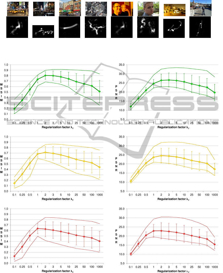
The diagrams in Fig. 5 show the mean MSSIM

and PSNR (thick line) for various noise levels, aver-

aged over the entire set of images and as a function of

the regularization parameter λ

∇

. The thin lines repre-

sent the maximum and minimum MSSIM and PSNR

values of all 8 images, and the error bars denote the

sample standard deviations. On average and also sub-

jectively, best results were obtained for λ

∇

between

0.5 and 2.5 depending on the noise level.

The paper by (Joshi et al., 2009) suggests a re-

duced regularization factor, λ

∇

, in the initialization

phase of the sparse prior in order to preserve de-

tails. Then, λ

∇

can be increased, once the penalty

terms based upon the two-color model become ac-

tive. However, their proposed values are inconsis-

RemovingMotionBlurusingNaturalImageStatistics

129

A~x = join







−1

| {z }

Data likelihood

+λ

∇

∑

∇,k

{z }

Sparse prior



· ext( j,~x)





j ∈ {R, G,B}



+ 2λ













| {z }

Alpha prior

+2λ







(~p

−

)

(~p

−

)

(~p

−

)

(~p

−

)







| {z }

d penalty term

∈ R

δ = join





j, C

−1

· ext( j,

| {z }

Data likelihood





j ∈ {R, G,B}



+ 2λ













| {z }

Alpha prior

+2λ







(~p

−

)

(~p

−

)

(~p

−

)

(~p

−

)







| {z }

d penalty term

∈ R

Figure 3: Combining the color and sparse priors within the IRLS optimization framework.

tent: λ

∇

= 0.25 followed by λ

∇

= 0.5 is mentioned

at one occasion, λ

∇

= 1 at another. This approach

can be problematic if the initial λ

∇

is chosen too low

(e.g. λ

∇

= 0.8). Details are preserved, but also arti-

facts within near-to homogeneous regions are intro-

duced as can be deduced from Fig. 5. Here, the

thin curves denoting the absolute minima of MSSIM

values are signiﬁcantly worse than their overall mean

substracted by their standard deviation (whereas this

gap is not observable for the maximum value curves;

this observation is only true up until λ

∇

= 1.0). On

the other hand, a high regularization factor such as

∇

= 3.0 over-smoothes the image. We therefore sug-

gest a nearly constant regularization factor for the gra-

dient prior. E.g., for a noise standard deviation of

σ = 2.5%, λ

∇

might initially be set to 1.5 and then be

increased to 2. Note that λ

∇

= 2 is slightly above the

optimal value discovered for this noise level in Fig. 5;

experience shows, though, that rather smooth images

require a slightly higher λ

∇

4 EVALUATION

First, we discuss the effects of the color prior and then

we show some qualitative results.

4.1 Understanding the Color Prior

In order to better understand the practical implications

of the two-color model, we show some segmentation

into primary and secondary colors in Fig. 6. The

original image is decomposed by EM clustering of

a 5 × 5 pixel neighborhood into a layer of primary

colors (Fig. 6(b)) and secondary colors (Fig. 6(c)).

The two-color model applies only at pixels where the

color difference between both layers is large enough.

Fig. 6(a) shows in black where the two-color model

does apply, and in white where the priors derived from

this model cannot be utilized. In these cases, a dif-

ferent kind of prior, e. g. a gradient prior, must be

used. (Joshi et al., 2009) suggest to generally com-

bine both a sparse gradient prior and the two-color

model (where applicable) with a reduced regulariza-

tion factor for the former.

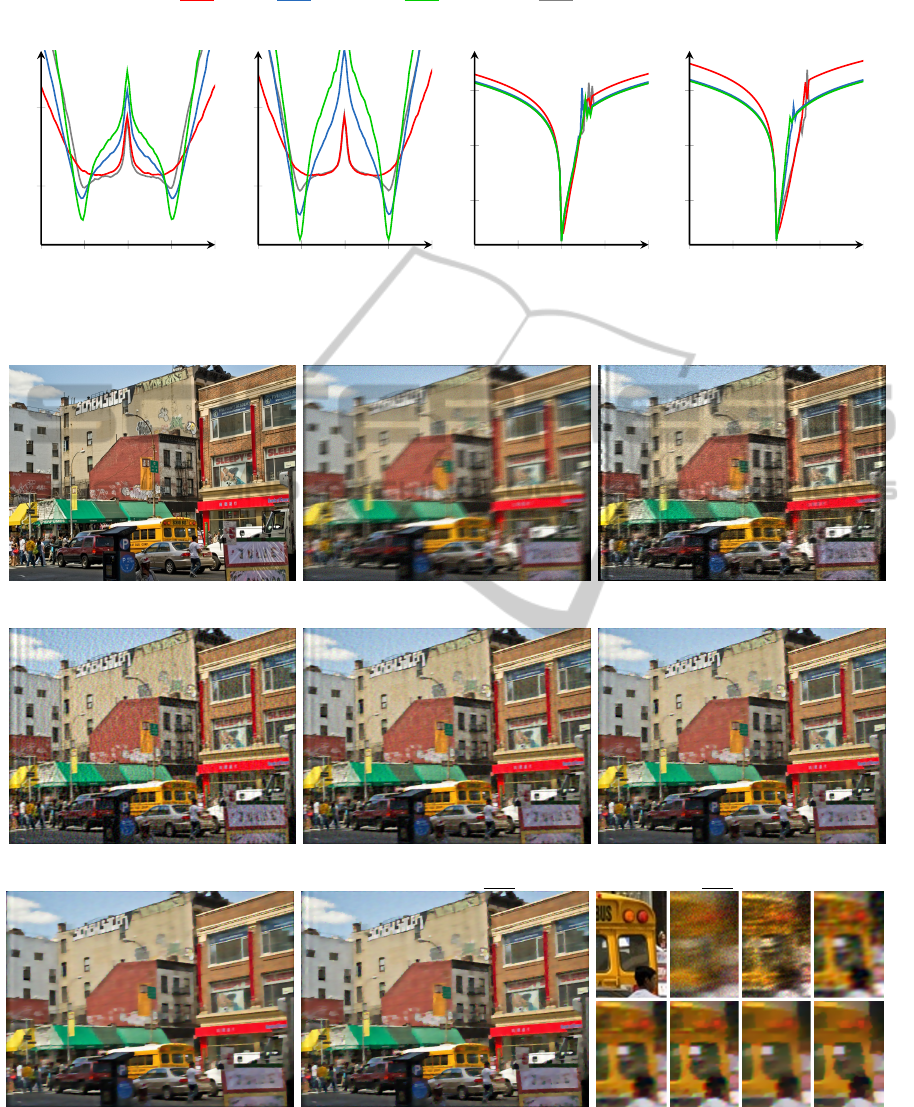
The histograms of the negative log-likelihoods in

Fig. 7 illustrate the effect of the alpha prior penalty

term on the distribution of alpha values. Both ex-

ample images have been initially deconvolved with a

sparse prior (λ

∇

= 2, γ = 0.5) before enabling the two-

color model (λ

= 5 for the ﬁrst image, and λ

= 100

for the second which ampliﬁes the effect for illustra-

tion purposes; λ

= 0). The red line shows the dis-

tribution after the initial sparse prior deconvolution.

The blue and green lines show the distribution after

1, respective 2, further IRLS iterations with the now

ICPRAM2014-InternationalConferenceonPatternRecognitionApplicationsandMethods

130

(a)  (b)  (c)  (d)  (e)  (f)  (g)  (h) 

Figure 4: Ground truth pictures and their accompanying blur kernels. Image sizes are approx. 800 × 600 pixels and blur

kernels are 27 × 27, 49 × 29, 31 × 31, 39 × 39, 27 × 27, 29 × 29, 51 × 45, 95 × 95, respectively.

(a) Noise standard deviation σ = 1%

(b) Noise standard deviation σ = 2.5%

Figure 5: Average MSSIM and PSNR values for the evaluation image set with its paired blur kernels of Fig. 4 at three different

noise levels σ as a function of the regularization parameter λ

∇

RemovingMotionBlurusingNaturalImageStatistics

131

(a) Two-color mask

(b) Primary colors (c) Secondary colors

Figure 6: Exemplary two-color model for the ground truth

image of Fig. 4(c). The two-color mask shows where the

color prior can be applied.

active alpha prior, while retaining sparse prior regu-

larization. The grey line, in comparison, illustrates

how the ﬁnal distribution would have looked like if

the alpha prior was never activated. Note how the

shown distributions have a shape similar to the ones

from Fig. 2(c), which is because the k-means only

algorithm without EM reﬁnement was used here to

construct the color model. In comparison with the

prior on distances d

, the alpha prior is more effective.

Both penalty terms require surprisingly large regular-

ization factors, especially compared to the parameters

mentioned by (Joshi et al., 2009).

In Fig. 10, we show the effects of different

amounts of regularization by λ

. The color noise

in the right Fig. 10(c) might indicate too few it-

erations with the sparse prior before the ﬁrst color

model was built by EM clustering. Hence, this result

with stronger regularization is not necessarily worse:

Some edges, e. g. at the perimeter of the blue parking

meter sign, or the white grafﬁti at the building wall

in the background, appear more clearly deﬁned with

larger λ

. If λ

becomes too large, the edges become

jagged and the image more and more resembles the

primary color layer. Strongly structured images with

lots of edges seem to proﬁt more from the prior on

alpha values. Unlike the sparse prior, there is no rec-

ommendation for the choice of λ

. Hence, some ex-

perimentation is required for each individual image.

4.2 Qualitative Evaluation

We show exemplarily qualitative results in Fig. 8 and

Fig. 9, whereby the second example is an image of

much less texture than the ﬁrst image, and also it has

much more noise added. Therefore the quality met-

rics show better values for the second example. An-

other reason for that can be found in the different blur

kernels which are shown in Fig. 4. The second exam-

ple is convolved with a PSF that has a weaker ridge

along its motion path with only two achnor points,

whereas the ﬁrst example has a PSF with a stronger

ridge that is equally thick along its whole motion path.

Therefore, the ﬁrst PSF mixes more pixels and it is

more ill-posed to deconvolve. On the other hand, the

second PSF mixes two locally aggregated clusters of

pixels (due to its two main anchor points) which are

seperated relatively far from each other. It can be seen

in both cases that the Gaussian prior performs bet-

ter than Richardson-Lucy, although it does not even

conform with the real kurtotic model of the gradi-

ent distribution. The Gaussian prior was only justi-

ﬁed because it is inexpensive to compute. But still its

smoothing capabilities successfully reduce noise and

hence outperform Richardson-Lucy. As expected, the

Laplacian prior performs a little better but at the cost

of much higher computation time. The sparse prior is

in most cases an enhancement over the Laplacian, and

as shown, even sub-optimal parameters tend to give

good results. The color prior again adds more com-

putational costs, but only minor improvements can

be visually recognized, like some sharper edges and

slightly reduced color noise, in the results of Fig. 8.

The quantitative metrics are even a little worse when

the color prior is enabled. The border effects in the de-

convolution results are common artifacts which (Zhou

et al., 2014) claims to reduce.

5 CONTEXT-ADAPTIVE PRIOR

Our experiments with the sparse priors suggest that

these tend to oversmooth the result image if the cho-

sen regularization factor λ

∇

is too large, and on the

other hand produce a noisy result image if λ

∇

is too

small. We therefore suggest a variable regularization

that can adapt to local image structure. This would

allow the user to have more control over the trade-

off between regularization blur and noise, by choos-

ing a stronger regularization in locally smooth image

regions where blur does not cause so much trouble,

and a weaker regularization in highly structured areas

(at the cost of introducing noise at these locations).

We experimentally study manual adaptation with user

ICPRAM2014-InternationalConferenceonPatternRecognitionApplicationsandMethods

132

Initial 1 iteration 2 iterations Sparse only result

−0.5

0.5

1.5

−ln p(α)

(a) Fig. 4(g), λ

= 5

−0.5

0.5

1.5

−ln p(α)

(b) Fig. 4(d), λ

= 100

−1

−0.5

0.5

−ln p(d)

= 5

−1

−0.5

0.5

−ln p(d)

(d) Fig. 4(d), λ

= 100

Figure 7: Effects of the alpha and distance penalty terms on images of Fig. 4(g) and Fig. 4(d).

(a) Ground truth image (b) Synthetically blurred image (c) Richardson-Lucy

MSSIM 0.455, PSNR 18.37 dB

(d) Gaussian prior: γ = 2, λ

∇

= 8

MSSIM 0.560, PSNR 20.43 dB

(e) Laplacian prior: γ = 1, λ

∇

= 2

MSSIM 0.605, PSNR 20.88 dB

(f) Sparse prior: γ = 0.5, λ

∇

= 1

MSSIM 0.618, PSNR 20.87 dB

(g) Sparse prior: γ = 0.5, λ

∇

= 2

MSSIM 0.585, PSNR 20.49 dB

(h) Color prior

γ = 0.5, λ

∇

= 2, λ

= 5, λ

= 5

MSSIM 0.602, PSNR 20.79 dB

(i) Cropped details, 4× enlarged

Figure 8: Deconvolution of the image of Fig. 4(c) with ground truth kernel and noise level σ = 5%.

RemovingMotionBlurusingNaturalImageStatistics

133

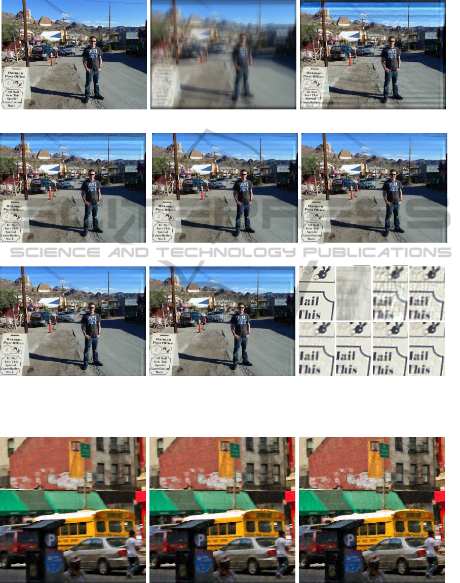
(a) Ground truth image (b) Synthetically blurred image (c) Richardson-Lucy

MSSIM 0.548, PSNR 18.62 dB

(d) Gaussian prior: γ = 2, λ

∇

= 9

MSSIM 0.599, PSNR 21.27 dB

(e) Laplacian prior: γ = 1, λ

∇

= 3

MSSIM 0.674, PSNR 23.48 dB

(f) Sparse prior: γ = 0.5, λ

∇

= 1.5

MSSIM 0.688, PSNR 23.72 dB

(g) Sparse prior: γ = 0.8, λ

∇

= 2.0

MSSIM 0.683, PSNR 23.70 dB

(h) Color prior

γ = 0.5, λ

∇

= 2, λ

= 1, λ

= 1

MSSIM 0.666, PSNR 22.59 dB

(i) Cropped details, 4× enlarged

Figure 9: Deconvolution of the image of Fig. 4(h) with ground truth kernel and noise level σ = 1%.

(a) λ

= 0.1 MSSIM 0.682, PSNR 22.15 dB (b) λ

= 2 MSSIM 0.685, PSNR 22.19 dB (c) λ

= 100 MSSIM 0.674, PSNR 21.86 dB

Figure 10: Deconvolution of the image of Fig. 4(c) with ﬁxed σ = 2.5%, λ

∇

= 2, λ

= 0 but varying λ

ICPRAM2014-InternationalConferenceonPatternRecognitionApplicationsandMethods

134

(a) Sketch (b) Edge map

(e) Ground truth (f) Blurry, σ = 2.5%

Figure 11: Locally varying vs. constant regularization of

the sparse prior, besides ground truth and blurry images.

intervention. The idea is to provide the user with ei-

ther the blurry image or, if the blur is too strong to be

able to recognize regions of salient structure, a rough

estimate of the deblurred image from the ﬁrst IRLS

iteration. The user can then paint over the edges and

other structured areas of the image to indicate weaker

regularization, as illustrated in Fig. 11(a). The lines

painted by the user can then be blurred slightly using

a Gaussian ﬁlter to make the change in regularization

less abrupt. The resulting image is then inverted and a

threshold is introduced so that the sketched areas also

experience a certain minimum amount of regulariza-

tion (e. g. at least 25% regularization in comparison to

areas where the user has indicated no important struc-

ture). This leads to an edge map like the one shown

in Fig. 11(b). The intensities resulting from this edge

map are then added as additional weights (multipliers)

∇,k,i

to the penalty terms ρ

∇

k,i

). The results shown

in Fig. 11 are encouraging. Recently, (Cui et al.,

2014) proposed a similar regularization approach as

an extension to Richardson-Lucy which is reported to

successfully reduce ringing artifacts.

6 CONCLUSIONS

On the basis of the work by (Levin et al., 2007b)

and their hyper-Laplacian penalty term, an extensi-

ble software framework for deconvolution using the

IRLS method has been developed. Because regular

photographs contain more than just intensity infor-

mation, a further regularization approach based upon

the two-color model proposed by (Joshi et al., 2009)

has been re-implemented and integrated into our op-

timization framework. In the evaluation part, we pro-

posed suitable regularization parameters for the pre-

sented penalty terms. Although enabling the addi-

tional color prior results in slightly sharper edges for

some images (e.g. Fig. 8), its huge computational

cost may not justify its general usage. Just using

the sparse gradient prior even with the faulty Gaus-

sian optimization model signiﬁcantly performs better

than Richardson-Lucy. With the additional computa-

tional cost when optimizing with a hyper-Laplacian

exponent that better models the kurtotic shape of

the sparse gradient distribution in an image, the de-

convolution results take another signiﬁcant leap for-

ward. Finally, our experimental work showed that fur-

ther context-adaptive regularization of gradient priors

seems promising in avoiding over-smoothing. The

presented deconvolution approach is robust in terms

of image noise but performs poorly in case the blur

kernel is not perfectly estimated (Zhong et al., 2013).

REFERENCES

Cecchi, G. A., Rao, A. R., Xiao, Y., and Kaplan, E. (2010).

Statistics of natural scenes and cortical color process-

ing. Journal of Vision, 10(11):1–13.

Chan, T. and Shen, J. (2005). Image Processing And Anal-

ysis: Variational, Pde, Wavelet, And Stochastic Meth-

ods. Siam.

Cho, S., Wang, J., and Lee, S. (2012). Video deblurring for

hand-held cameras using patch-based synthesis. ACM

Trans. on Graphics, 31(4):64:1–64:9.

Cui, G., Feng, H., Xu, Z., Li, Q., and Chen, Y. (2014). A

modiﬁed Richardson–Lucy algorithm for a single im-

age with adaptive reference maps. Optics & Laser

Technology, 58:100–109.

Dong, W., Feng, H., Xu, Z., and Li, Q. (2012a). Blind image

deconvolution using the ﬁelds of experts prior. Optics

Communications, 285:5051–5061.

Dong, W., Shi, G., Li, X., Zhang, L., and Wu, X. (2012b).

Image reconstruction with locally adaptive sparsity

and nonlocal robust regularization. Image Communi-

cation, 27:1109–1122.

Faraway, J. J. (2002). Practical regression and

ANOVA using R. Online. http://cran.r-project.org/

doc/contrib/Faraway-PRA.pdf.

RemovingMotionBlurusingNaturalImageStatistics

135

Gentle, J. (2007). Matrix algebra: theory, computations,

and applications in statistics. Springer texts in statis-

tics. Springer, New York, NY.

Gupta, A., Joshi, N., Zitnick, L., Cohen, M., and Curless, B.

(2010). Single image deblurring using motion density

functions. In ECCV ’10: Proc. of the 10th Europ.

Conf. on Comp. Vision.

Huang, J. (2000). Statistics of natural images and models.

PhD thesis, Brown Univ., Providence.

Ito, A., Sankaranarayanan, A. C., Veeraraghavan, A., and

Baraniuk, R. G. (2013). Blurburst: Removing blur due

to camera shake using multiple images. ACM Trans.

Graph. Submitted.

Ji, H. and Wang, K. (2012). A two-stage approach to blind

spatially-varying motion deblurring. In IEEE Conf.

on Comp. Vision and Pattern Recogn. (CVPR), pages

73–80. IEEE Comp. Soc.

Joshi, N., Zitnick, C., Szeliski, R., and Kriegman, D.

(2009). Image deblurring and denoising using color

priors. In IEEE Conf. on Comp. Vision and Pattern

Recognition (CVPR), pages 1550–1557. IEEE Comp.

Soc.

Krishnan, D. and Fergus, R. (2009). Fast image deconvo-

lution using hyper-laplacian priors. In Neural Inform.

Proc. Sys.

Levin, A., Fergus, R., Durand, F., and Freeman, W. T.

(2007a). Deconvolution using natural image priors.

Technical report, MIT.

Levin, A., Fergus, R., Durand, F., and Freeman, W. T.

(2007b). Image and depth from a conventional camera

with a coded aperture. ACM Trans. Graph., 26.

Levin, A. and Weiss, Y. (2007). User assisted separation

of reﬂections from a single image using a sparsity

prior. IEEE Trans. Pattern Anal. and Mach. Intell.,

29(9):1647–1654.

Li, X., Pan, J., Lin, Y., and Su, Z. (2013). Fast blind deblur-

ring via normalized sparsity prior. Journal of Inform.

& Comp. Sc., 10(16):5083–5091.

Lin, H. T., Tai, Y.-W., and Brown, M. S. (2011). Motion reg-

ularization for matting motion blurred objects. IEEE

Trans. Pattern Anal. and Mach. Intell., 33(11):2329–

2336.

Liu, R., Li, Z., and Jia, J. (2008). Image partial blur de-

tection and classiﬁcation. In IEEE Conf. on Comp.

Vision and Pattern Recognition (CVPR), pages 1–8.

IEEE Comp. Soc.

Marichal, X., Ma, W.-Y., and Zhang, H.-J. (1999). Blur

determination in the compressed domain using DCT

information. In Intern. Conf. on Image Proc. (ICIP),

pages 386–390.

Meer, P. (2004). Robust techniques for computer vision.

In Medioni, G. and Kang, S. B., editors, Emerging

Topics in Computer Vision, chapter 4. Prentice Hall

PTR, Upper Saddle River, NJ.

Scales, J. A. and Gersztenkorn, A. (1988). Robust methods

in inverse theory. Inverse Problems, 4(4):1071.

Scales, J. A., Gersztenkorn, A., and Treitel, S. (1988). Fast

solution of large, sparse, linear systems: Applica-

tion to seismic travel time tomography. Journal of

Computational Physics, 75:314–333.

Schmidt, U., Rother, C., Nowozin, S., Jancsary, J., and

Roth, S. (2013). Discriminative non-blind deblurring.

In IEEE Conf. on Comp. Vision and Pattern Recogni-

tion (CVPR), pages 604–611. IEEE Comp. Soc.

Schmidt, U., Schelten, K., and Roth, S. (2011). Bayesian

deblurring with integrated noise estimation. In

IEEE Conf. on Comp. Vision and Pattern Recognition

(CVPR), pages 2625–2632. IEEE Comp. Soc.

Shi, M.-z., Xu, T.-f., Feng, L., Liang, J., and Zhang, K.

(2013). Single image deblurring using novel image

prior constraints. Optik - International Journal for

Light and Electron Optics, 124(20):4429–4434.

Simoncelli, E. (1997). Statistical models for images: Com-

pression, restoration and synthesis. In In 31st Asilo-

mar Conf on Signals, Systems and Computers, pages

673–678. IEEE Comp. Soc.

Sorel, M. and Sroubek, F. (2012). Restoration in the pres-

ence of unknown spatially varying blur. In Gunturk,

B. and Li, X., editors, Image Restoration: Fundamen-

tals and Advances, pages 63–88. CRC Press.

Srivastava, A., Lee, A. B., Simoncelli, E. P., and c. Zhu, S.

(2003). On advances in statistical modeling of natural

images. Journal of Math. Imaging and Vision, 18:17–

33.

Wang, S., Hou, T., Border, J., Qin, H., and Miller, R.

(2012). High-quality image deblurring with panchro-

matic pixels. ACM Trans. Graph., 31(5).

Wang, Z., Simoncelli, E. P., and Bovik, A. C. (2003). Multi-

scale structural similarity for image quality assess-

ment. In Proc. of the 37th IEEE Asilomar Conf. on

Signals, Systems and Computers.

Weiss, Y. and Freeman, W. (2007). What makes a good

model of natural images? In IEEE Conf. on Comp.

Vision and Pattern Recognition (CVPR), pages 1–8.

IEEE Comp. Soc.

Whyte, O., Sivic, J., Zisserman, A., and Ponce, J. (2012).

Non-uniform deblurring for shaken images. Intern.

Journal of Comp. Vision, 98(2):168–186.

Yuan, L., Sun, J., Quan, L., and Shum, H.-Y. (2007).

Blurred/non-blurred image alignment using sparse-

ness prior. In Proc. of the 11th Intern. Conf. on Comp.

Vision (ICCV), pages 1–8.

Yun-Fang, Z. (2010). Blur detection for surveillance video

based on heavy-tailed distribution. In Asia Paciﬁc

Conf. on Postgrad. Research in Microelectronics and

Electronics, pages 101–105.

Zhong, L., Cho, S., Metaxas, D., Paris, S., and Wang, J.

(2013). Handling noise in single image deblurring us-

ing directional ﬁlters. In IEEE Conf. on Comp. Vision

and Pattern Recogn. (CVPR), pages 612–619. IEEE

Comp. Soc.

Zhou, X., Zhou, F., Bai, X., and Xue, B. (2014). A bound-

ary condition based deconvolution framework for im-

age deblurring. Journal of Computational and Applied

Mathematics, 261:14–19.

ICPRAM2014-InternationalConferenceonPatternRecognitionApplicationsandMethods

136