A Stochastic Programming Approach for Stafﬁng and Scheduling Call

Centers with Uncertain Demand Forecasts

Mathilde Excofﬁer

, C

eline Gicquel

, Oualid Jouini

and Abdel Lisser

Laboratoire de Recherche en Informatique - LRI, Orsay, France

Ecole Centrale Paris - ECP, Ch

atenay-Malabry, France

Keywords:

Call Centers, Queuing Systems, Stochastic Optimization, Joint Chance Contraints, Stafﬁng, Shift-Scheduling.

Abstract:

We consider a workforce management problem arising in call centers, namely a stafﬁng and shift-scheduling

problem. It consists in determining the minimum-cost number of agents to be assigned to each shift of the

scheduling horizon so as to reach the required customer quality of service. We assume that the mean call

arrival rate in each period of the horizon is a random variable following a continuous distribution. We model

the resulting optimization problem as a stochastic program involving joint probabilistic constraints. This

allows to manage the risk of not reaching the required quality of service at the horizon level rather than on a

period by period basis. We propose a solution approach based on linear approximations to provide approximate

solutions of the problem. We ﬁnally give numerical results carried out on a real-life instance. These results

show that the proposed approach compares well with previously published approaches both in terms of risk

management and cost minimization.

1 INTRODUCTION

Stafﬁng and shift-scheduling in call centers is a very

challenging problem in Operations Research. Call

centers are expensive infrastructures for companies,

in which the staff agents represent 60% to 80% of the

total operating budget (Aksin et al., 2007).Thus an ef-

ﬁcient workforce management is of primary impor-

tance to achieve proﬁtability of a call center. One of

the most important problem is the short-term stafﬁng

and scheduling problem: it consists in deciding how

many staff members handling the phone calls, i.e.

”agents”, should work during the forthcoming days

or weeks in order to minimize manpower costs while

ensuring that the required customer quality of service

is reached. The Quality of Service (QoS) can be for

instance a maximum expected abandonment rate, ie

number of clients hanging up without being served,

or a maximum expected waiting time before entering

service in the queue.

The problem here is to decide how many people

answering the phone, that is to say agents, we need to

assign each day. This problem comprises two steps.

The ﬁrst step is the stafﬁng problem, which in-

volves computing the number of required agents.

These values come from a calculation based on an ob-

jective service level and estimations of arrival rates.

The objective service level considered here is the

maximum expected time of waiting before being

served. The estimations of arrival rates come from

forecasts using historical data, in which usually the

main (and often only) information available is the

number of calls per period. As arrival rates strongly

vary in time, estimations are given for short periods

of time (usually 30-minute periods).

In order to use all this information and compute

the values of required agents at each period, we model

the call center at each period as an Erlang C queuing

system in stationary state and we use the Erlang C

results, as commonly done practice.

The second step is the scheduling problem. This

optimization problem involves scheduling enough

agents with respect to a given Quality of Service

(QoS) while respecting the inherent constraints of

manpower work, like hiring a whole number of

agents, or following some working hours. The goal

here is to assign established shifts to the working

agents through a ﬁven period.

There are several criteria in the establishment of the

problem:

• Uncertainty Management: how uncertainty is

dealt with in the model?

• Risk Management: how to modelize the penalty

Excofﬁer M., Gicquel C., Jouini O. and Lisser A..

A Stochastic Programming Approach for Stafﬁng and Scheduling Call Centers with Uncertain Demand Forecasts.

DOI: 10.5220/0004832100800088

In Proceedings of the 3rd International Conference on Operations Research and Enterprise Systems (ICORES-2014), pages 80-88

ISBN: 978-989-758-017-8

 2014 SCITEPRESS (Science and Technology Publications, Lda.)

of not reaching the expected QoS?

• Recourse: what possibility do we have to correct

the solution in a second-stage after observation?

Several approaches for stafﬁng call centers con-

sidering uncertainty of arrival rates forecasts exist

in the literature. (Jongbloed and Koole, 2001) fo-

cus on giving a prediction interval for possible ar-

rival rates, and then give an interval for the associate

required numbers of agents. (Gurvich et al., 2010)

present and compare two different approaches for

dealing with uncertainty: the average-performance

constraints problem considers the average of the un-

certain variables and the chance constraints problem

deals with uncertainty and risk both together.

(Robbins and Harrison, 2010) choose to model

the mixed integer linear program with several scenar-

ios each deﬁning a probability of reaching the QoS.

Moreover, they use piecewise linear approximations

of their QoS function. The idea of using scenarios

through discretization of the probability distributions

is used in several papers, such as (Liao et al., 2012)

and (Gans et al., 2012) for example, or (Luedtke et al.,

2007) who consider a ﬁnite distribution from the be-

ginning.

The risk management can be modeled by a penalty

cost in the objective function, as in (Robbins and Har-

rison, 2010), or with joint chance constraints pro-

grams, as in (Gurvich et al., 2010).

(Liao et al., 2013) introduce a distributionally

robust approach for the scheduling problem and use

discrete distributions for uncertainty.

While (Robbins and Harrison, 2010), (Liao et al.,

2012) and (Gurvich et al., 2010) use a one-stage

approach, (Mehrotra et al., 2009), (Gans et al., 2012)

and (Erdo

gan and Iyengar, 2007) allow a recourse on

the solution, with a two-stage approach.

The contributions of the present paper are thus

threefold. First, we model the call arrival rate

in each period as a random variable following a

continuous normal distribution. This is in contrast

with most previously published approaches which

rely on a discrete representation of the uncertainty

through a ﬁnite set of scenarios. Since we consider

every possible variation of the arrival rate instead

of a limited number, our approach leads to a better

accuracy of the ﬁnal solution. Moreover, we keep this

idea of continuity during all the process until the ﬁnal

solving of the linear programs. Second, we propose a

solution in order to solve the stafﬁng problem and the

shift-scheduling problem as a one-stage stochastic

program involving joint probabilistic constraints. It

allows to manage the risk of not reaching the required

quality of service at the scheduling horizon level

rather than on a period by period basis. Moreover,

our approach relies on a dynamic sharing out of

the risk among all the periods and thus provides

ﬂexibility in the risk management. Third we present

a linear-approximation based solution approach

leading to approximate solutions for the problem.

The rest of this paper is organized as follows. In

Section 2 we describe the call center queuing model.

In Sections 3 and 4 we present our approach to model

and solve the stochastic stafﬁng and shift-scheduling

problem. First we deﬁne the joint chance constraints

program and then we linearize the inverse of the cu-

mulative distribution function in the constraints. Then

we give in Section 5 computational results on several

instances and we compare them to results given by

simpler models. Finally we conclude and highlight

future research in Section 6.

2 STAFFING PROBLEM

MODELING

The problem here is to decide how many people an-

swering the phone, that is to say agents, we need to

assign each day. In order to do that, we are given a

number of required agents. These values of require-

ments come in fact from a calculation based on an

objective service level and estimations of arrival rates.

The objective service level is the customer Quality of

Service. The estimations of arrival rates come from

forecasts using historical data. As arrival rates vary in

time, estimations are given for short periods of time,

eg. 30 minute-periods.

In order to compute the values of required agents

at each period, we model the call center as a queueing

system in stationary state and we use the Erlang C

model.

Call centers are typically modeled as queuing sys-

tems as we can see for example in (Gross et al., 2008).

The day is divided into T periods. During each pe-

riod, we assume that the stationary regime is reached.

Customer arrival process during each period is Pois-

son and service times are assumed to be independent

and exponentially distributed with rate µ. This is a

non-stationary queue M

/M/N

where N

represents

the number of servers, i.e. the number of agents in

our problem.

Customers are served in the order of their arrivals,

i.e. under the First Come-First Served (FCFS) disci-

pline of service. The queue capacity is assumed to be

inﬁnite. Finally, customers abandonment and retrials

are ignored.

AStochasticProgrammingApproachforStaffingandSchedulingCallCenterswithUncertainDemandForecasts

Since we consider uncertainty on arrival rates, we

have to deal with stochastic programs. We assume

that the arrival rates are random variables, denoted

by Λ

for the period t, following normal distributions

where the expected values are the forecast values.

3 PROBLEM FORMULATION

We propose here to describe and solve a mixed integer

linear stochastic program able to solve a joint stafﬁng

and scheduling problem.

As explained, we consider that the values we use are

forecasts obtained from historical data and may differ

from the reality. We still want to guarantee a Qual-

ity of Service, expressed with a risk of how much can

be the forecasts and reality different. In order to deal

with a global problem, this risk will be set for the en-

tire horizon (for example one week or one month).

In Section 2 we explained that we computed the

number of required agents for each 30-minute-period

(or 1-hour). We create several possible shifts, accord-

ing to real work days, which cover the schedule of

the call center. As it is inconvenient to ask an agent

to come for only short periods of time, they have

to follow typical shifts (like full-time or part-time).

This may lead to over-stafﬁng on some periods. In

this model we consider shifts with breaks, like lunch

breaks.

We want to deﬁne a risk level for the whole hori-

zon. In order to deal with this condition, we model

our problem with joint chance constraints (Pr

ekopa,

2003):

min c

x (1)

s.t. P{Ax > B} > 1 − ε

∈ Z

,ε ∈]0;1]

where x is the agents vector, and x

is the number of

agents assigned to the shift i ; c is the cost vector and

A = (a

i, j

) is the matrix of shifts for i ∈ [[1; T ]] and

j ∈ [[1;S]]. The vector B is the vector of the staffed

agents random variables B

This program optimizes the cost of hired agents

under the constraint that the probability of reaching

the requirement for the whole schedule is higher than

the quality interval 1 − ε.

We denote by A the matrix of possible shifts. The

term a

i, j

is equal to 1 if agents working during period i

according to shift j and 0 if not. Thus Ax is the vector

deﬁning the number of agents working at each period.

The variables B

are computed with an Erlang C

model. The arrival rates values are independent ran-

Figure 1: Example of a simple shifts matrix.

dom variables following continuous normal distribu-

tions for which the means are the forecast values.

Since the B

are function of Λ

, they are random vari-

ables.

Thus we now consider B a vector of random

variables ; for each period t, B

is function of the

arrival rate Λ

, and so we have to deal with the

unknown continuous distribution of B

Since we consider independent random variables,

we split the product of probabilities and obtain the

following Mixed Integer Program:

min c

x (2)

s.t.

∏

t=1

∗ x) > (1 − ε)

∈ Z

,ε ∈]0;1]

where A

is the t-th row of A matrix and

∗ x) = P(B

6 A

∗ x).

In order to solve this program, we need to sepa-

rate the chance constraint into several constraints for

each period. This means dividing up the risk along

the horizon.

The simplest way is equally dividing the risk

through the T periods, according to Bonferroni

method:

min c

x (3)

s.t. ∀t ∈ [[1; T ]], (A

x) > F

−1



(1 −ε)



∑

t=1

= 1

∈ Z

,ε ∈]0;1],∀t ∈ [[1;T ]], y

∈]0;1]

We divide the quality interval and then apply

the inverse of the normal cumulative distribution

function. The drawback of this idea is that we have

to decide how to distribute the risk in advance, before

the optimization process.

ICORES2014-InternationalConferenceonOperationsResearchandEnterpriseSystems

In order to be able to optimize the risk through the

periods, we decide to include the sharing out of the

risk in the optimization and put the risk levels as prob-

lem variables. Instead of considering

as the propor-

tion of the risk for one period, we introduce propor-

tion variables denoted as y

. They are now variables

and the sum of y

still should be 1 in order to reach

the global risk level.

The new problem, with a ﬂexible sharing out of

the risk is now:

min c

x (4)

s.t. ∀t ∈ [[1; T ]], (A

x) > F

−1

((1 −ε)

)

∑

t=1

= 1

∈ Z

,ε ∈]0;1],∀t ∈ [[1;T ]], y

∈]0;1]

In order to solve this problem, we propose two lin-

earizations which give an upper bound and a lower

bound. These linearizations are based on piecewise

approximations of y 7→ F

−1

). We cannot compute

exact values of this function, thus we focus on linear

approximations. This function is continuous and dif-

ferentiable (except on a countable number of points).

We need to deal with a convex function in order to

apply the approximations.

4 SOLUTION APPROXIMATIONS

4.1 Deﬁnition of ψ Function

We ﬁrst introduce the function ψ which gives a re-

lation between b and λ. We consider the following

continuous function ψ:

ψ :R →R

(5)

λ 7→ψ(λ) = b(λ, ASA

∗

,µ)

The function ψ gives the minimum number of

agents b required to ensure that the targeted QoS ASA

∗

is reached when the call arrival rate is λ and the ex-

pected service rate is µ. The chosen QoS is the Aver-

age Speed of Answer (ASA). The computed value of

b is a real number and not an integer, which is nec-

essary to allow the linear approximations in the next

parts: we need the inverse of the cumulative distribu-

tion function to be continuous.

To the best of our knowledge, an analytical ex-

pression computing ψ is not known. However, for a

given value of λ, we propose to compute ψ(λ) with

the following algorithm.

First we consider this well-known Erlang C

model’s function:

ASA(N,λ,µ) = E[Wait] (6)

N ∗ µ ∗ (1 −

N∗µ

)



1 +(1 −

N∗µ

)

N−1

∑

m=0

(

)

N−m



This formula gives the expectation of waiting time

(ASA: Average Speed of Answer) given the arrival

rate λ, the service rate µ and the number of servers N

which is an integer. In order to consider ψ as func-

tion of a positive real value of b, we use the algorithm

below:

• We compute ASA(N,λ,µ) and ASA(N + 1,λ,µ)

such that

ASA(N,λ,µ) > ASA

∗

and ASA(N +1,λ,µ) < ASA

∗

We denote ASA(N,λ,µ) as ASA

N,λ

• The real value of N is computed by a linearization

in the [ASA

N,λ

;ASA

N+1,λ

] segment. The afﬁne

function is:

ASA

∗

=(ASA

N+1,λ

− ASA

N,λ

) ∗b

+ (N +1) ∗ ASA

N,λ

− N ∗ ASA

N+1,λ

and b is the real value ψ(λ) we are looking for. 

Using this algorithm for the value of λ we are consid-

ering in the ψ function, ﬁnally we obtain b.

ψ(λ) = b (7)

ASA

∗

+ N ∗ ASA

N+1,λ

− (N +1) ∗ ASA

N,λ

ASA

N+1,λ

− ASA

N,λ

The ψ function allows us to determine the values

of b as a function of λ, µ and an objective QoS ASA

∗

In a nutshell, we determine the number of agents re-

quired to deal with the arrival rates of clients λ with

respecting a Quality of Service previously deﬁned.

This function is strictly increasing.

We can denote then

(b) = F

(ψ

−1

(b))

4.2 Convexity of y 7→ F

−1

)

We have previously deﬁned F

(b) = F

(ψ

−1

(b)).

Thus we have

(b) = F

(ψ

−1

(b)) = 1 − ε (8)

and so

−1

(1 −ε) = ψ(F

−1

(1 −ε)) (9)

AStochasticProgrammingApproachforStaffingandSchedulingCallCenterswithUncertainDemandForecasts

In our problem, we split the risk 1−ε. Since 1 − ε

represents a probability, let’s call it p in this part. In

our problem we want a high quality interval and thus

a small value of ε. We can consider from here that

p > 0.5, which is necessary for the following proof of

convexity.

We need to consider p

,y ∈]0;1] in our optimiza-

tion problem. So we consider the equality

−1

) = ψ(F

−1

))

with y ∈]0; 1].

Lemma Since f : y 7→ p

is convex and

g : p 7→ F

−1

(p) is convex for p > 0.5 and in-

creasing, thus y 7→ F

−1

) is convex.

Proof

∀p ∈ [0; 1],∀(x,y) ∈ [0;1], ∀t ∈ [0; 1],

f (tx + (1 −t)y) 6 t ∗ f (x) + (1 − t) ∗ f (y)

g( f (tx + (1 − t)y)) 6 g(t ∗ f (x) + (1 − t) ∗ f (y))

6 t ∗ g( f (x)) + (1 −t) ∗ g( f (y))

(10)

−1

tx+(1−t)y

) 6 tF

−1

) +(1 −t)F

−1

)



This previous result and the strictly increasing

function λ 7→ ψ(λ) helped us to note that y 7→ F

−1

)

is a generally convex function. We then consider an

approximated function of y 7→ F

−1

) which is con-

vex.

With this result we are able to linearize the ap-

proximated convex function as in (Cheng and Lisser,

2012).

4.3 Piecewise Linear Approximation

Here we give an upper approximation of

y 7→ F

−1

Let y

∈]0;1], j ∈ [[1; n]] be n points such that y

< ... < y

Let’s denote

−1

B j

) the linearized approxima-

tion of F

−1

) between y

and y

j+1

∀ j ∈ [[1; n − 1]], (11)

−1

B j

) =F

−1

)

y −y

j+1

− y

−1

j+1

) −F

−1

))

= δ

∗ y + α

Since F

(b) = F

(ψ

−1

(b)), we have

∀p ∈]0;1[, F

−1

B j

(p) = ψ(F

−1

Λ j

(p))

Thus the coefﬁcients are:

ψ(F

−1

Λ j

j+1

) −ψ(F

−1

Λ j

))

j+1

− y

(12)

=ψ(F

−1

)) −y

∗ δ

(13)

Because of the convexity of the approximation, the

condition in our program would be:

∀y ∈]0; 1],

−1

) = max

j∈[[1;n−1]]

{

−1

B j

)} (14)

So our approximated program is now:

min c

x (15)

s.t. ∀t ∈ [[1; T ]],∀ j ∈ [[1;n −1]], A

x > α

+ δ

∗ y

∑

t=1

= 1

∀i ∈ [[1;S]],x

∈ Z

,∀t ∈ [[1; T ]],y

∈]α

;1]

with n points for linear approximation with

(α

,δ

) coordinates. S is the number of shifts and T

the total number of periods.

4.4 Piecewise Tangent Approximation

Let’s now express a lower approximation of y 7→

−1

Let y

∈]0;1], j ∈ [[1; n]] be n points such that y

< ... < y

We apply a ﬁrst-order Taylor series expansion

around these n tangents points. Let’s denote

−1

B j

)

the linearized approximation of F

−1

B j

) around y

Then

∀ j ∈ [[1; n]], (16)

−1

B j

) = F

−1

)

+ (y − y

)(F

−1

)

) ∗ln(p) ∗ p

= δ

∗ y + α

with

−1

)

) =

−1

)(p

)

−1

))

And since f

(b) =

(ψ

−1

(b))

(ψ

−1

(b))

as a deﬁnition of

composition of random variables:

ICORES2014-InternationalConferenceonOperationsResearchandEnterpriseSystems

−1

)(p

) =

(ψ

−1

)))

(ψ

−1

)))

(ψ

−1

(ψ(F

−1

))))

(ψ

−1

(ψ(F

−1

))))

−1

))

−1

))

The coefﬁcients are:

=ln(p) ∗ p

∗

−1

))

−1

))

(17)

=ψ(F

−1

)) −y

∗ δ

(18)

Again, the condition in our approximated program is:

−1

) = max

j∈[[1;n]]

−1

B j

)} (19)

Finally the piecewise tangent approximated pro-

gram is:

min c

x (20)

s.t. ∀t ∈ [[1; T ]],∀ j ∈ [[1;n]], A

x > α

+ δ

∗ y

∑

t=1

= 1

∀i ∈ [[1;S]],x

∈ Z

,∀t ∈ [[1; T ]],y

∈]0;1]

with n points for tangent approximation with

(α

,δ

) coordinates.

5 NUMERICAL EXPERIMENTS

5.1 Instance

We apply our model to an instance from a health in-

surance call center. We use 19 different shifts, both

full-time and part-time and consider the scheduling

for one week (5.5 days, from Monday to Saturday

midday).

We split the time horizon into 30-minute periods,

considering 10 hours a day from Monday to Friday

and 3.5 hours for Saturday morning, which gives 107

periods.

We consider that the agents are paid according to

the number of worked hours. The cost of one agent is

proportional to the number of periods worked. Thus

it depends on the shift the agent works on. Here we

set the cost to 1 for the fullest shifts (with the high-

est number of periods) and the costs of other shifts

are a strict proportionality of the number of worked

periods.

The data used to staff and shift-schedule are

arrival rates varying between 3 calls/min and 43

calls/min, following a typical daily seasonality, as

described in (Gans et al., 2003). We denote ∀t ∈

[[1; T ]],λ

the mean of the T random variables, which

are the given data. The variances σ

are random val-

ues generated between [

;

We apply the same instance to the programs (15)

and (20) and, as a comparison, to the program (3) in

which we divided the risk through the periods in a

pre-treatment.

5.2 Comparison with Other Programs

We also add the results from simple programs:

• In this approach we want to reach the risk level at

each period, not through the whole horizon:

min c

x (21)

s.t. ∀t ∈ [[1; T ]], P{A

x > b

} > 1 − ε

∈ Z

,ε ∈]0;1]

Thus we got this ﬁnal program:

min c

x (22)

s.t. ∀t ∈ [[1; T ]], (A

x) > F

−1

((1 −ε))

∑

t=1

= 1

∈ Z

,ε ∈]0;1]

• Finally we can compare with the results of the de-

terministic program:

min c

x (23)

s.t. ∀t ∈ [[1; T ]], (A

x) > b

∈ Z

The values of b

here are computed with the Er-

lang C formula using the mean forecasted values, con-

sidered as certains.

5.3 Results

We apply our models with the following parameters:

• µ = 1

• ASA

∗

= 1

• ε = 0.10

AStochasticProgrammingApproachforStaffingandSchedulingCallCenterswithUncertainDemandForecasts

Table 1: Result for stafﬁng and shift-scheduling.

Shi f t Deter Dis joint Fixed LowerB U pperB

1 0 0 0 0 0

2 0 0 0 0 0

3 0 0 0 0 0

4 0 0 0 0 0

5 0 0 0 0 0

6 2 2 1 1 1

7 0 0 0 0 0

8 0 0 0 0 0

9 0 0 0 0 0

10 0 0 0 0 0

11 13 14 18 18 19

12 9 10 9 9 12

13 5 6 8 9 11

14 0 1 3 2 4

15 5 6 7 6 3

16 6 7 8 7 7

17 0 0 0 0 0

18 4 5 6 4 3

19 4 4 5 4 3

Total 48 55 65 60 63

Cost f unction 47.44 54.44 64.72 59.72 62.72

In table 1 we show the solutions for stafﬁng and

shift-scheduling of this instance for 5 programs: col-

umn 1 gives the shift, column 2 (Deter) presents the

x vector obtained with the deterministic model (23),

column 3 (Disjoint) gives the results with the disjoint

chance constraints model (22) and column 4 (Fixed)

with the the ﬁxed-risked model (3). Finally, columns

5 (LowerB) and 6 (UpperB) present the results ob-

tained with the lower bound (20) and the upper bound

(15) approximations.

We used 5 points for computing both lower and

upper bounds. The gap between the two bounds is

D = 5%.

In order to check the efﬁciency of these solutions,

we randomly generated 100 scenarios according to

the historical data we previously used and checked the

feasibility of the 5 solutions. If the number of agents

required in at least one period of a scenario is insufﬁ-

cient, the latter is considered as violated.

In table 2 are the results for a batch of 100 scenar-

ios. JCC stands for ”Joint Chance Constraints”.

In the ﬁgure 2 we plotted for each model and each

scenario the difference between the number of agents

in the previous solutions and the number of agents ac-

tually needed b

present

− b

needed

. When this value is

negative for at least one period, the model is invali-

dated for the scenario.

Table 2: Percentage of violated scenarios.

Model % of violation

Deterministic model 100%

Disjoint chance constraints model 49%

JCC model with ﬁxed risk level 0%

JCC lower bound and ﬂexible risk 3%

JCC upper bound and ﬂexible risk 1%

Targeted maximal risk 5%

First we compare the schedules obtained by using

the various models discussed in the paper based on

the total stafﬁng cost.

We note that the deterministic (23) and disjoint

(22) models provide less expensive schedules than the

joint chance constraint models (15), (20) and (3).

However our approximated programs where the

risk is dynamically divided through the periods pro-

vide less expensive schedules than the joint chance

constraint model where the risk is a priori divided

equally between the scheduling periods (3). This

shows the interest of allowing some ﬂexibility in the

way the risk is allocated between the scheduling peri-

ods.

In small instances we could have chosen another

sharing out a priori of the risk (by analysing wisely

the risky periods) but it remains too complex on in-

stances like ours.

Second, we note that all the cheaper solutions than

the two bounds of our new model of joint chance con-

ICORES2014-InternationalConferenceonOperationsResearchandEnterpriseSystems

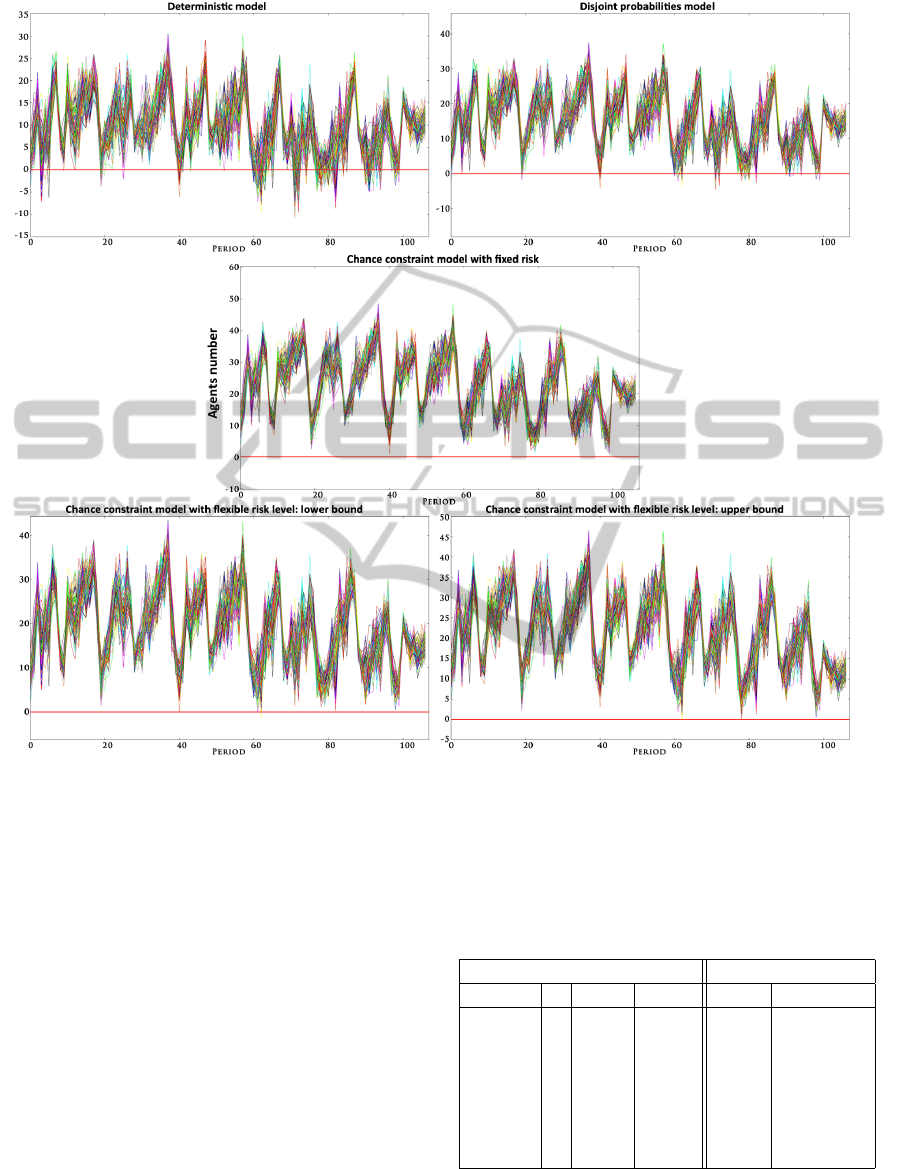
Figure 2: Violated scenarios for each model.

traints with a ﬂexible sharing out of the risk does not

validate the condition of the targeted QoS. Thus they

cannot be considered as possible alternatives. The ro-

bustness, i.e. the capability of providing the required

QoS over the whole scheduling horizon within the

maximum allowable risk level, is an essential crite-

rion and its validation is mandatory to approve the

model.

The last 3 programs which are joint chance con-

straints models are the only models respecting the ob-

jective service level. Our approximated programs are

cheaper than the joint chance constraints model with

a ﬁxed sharing out of the risk. Our approach allows us

to save between 3.2% (upper bound) and 8.4% (lower

bound) compared to this program.

This shows the practical interest of the proposed

modelling and solution approach as we provide ro-

bust schedules at a lesser cost than previously joint

constraint models.

In table 3, we present results for different values

of λ, µ, ASA

∗

and ε (illustrated in the table by the risk

interval).

Table 3: Results for different parameters.

Parameters Results

λ range µ ASA

∗

Risk ε Gap Violations

3 −43 1 1 10% 0.05 1 −3

3 −43 1 1 05% 0.04 1 −2

3 −43 2 1 30% 0.0 5 − 13

3 −43 1 2 30% 0.03 12 −18

6 −86 1 2 10% 0.004 5 −6

6 −86 1 1 10% 0.005 5 −6

6 −86 1 1 01% 0.003 0 −0

The ”Gap” column gives the gap between the

lower bound and the upper bound solutions. The ”vi-

olation” column gives the numbers of violated scenar-

AStochasticProgrammingApproachforStaffingandSchedulingCallCenterswithUncertainDemandForecasts

ios for the lower and the upper bounds. We note that

for higher values of λ, the bounds are really close and

give good results.

6 CONCLUSIONS

In this paper we proposed a new procedure for solving

the stafﬁng and shift-scheduling problem in one step

with uncertain arrival rates. We introduced the mod-

elization of arrival rates as continuous normal distri-

butions and we were able to propose linear approxi-

mations and upper and lower bounds for our stafﬁng

and shift-scheduling problem in call centers. The con-

struction of the ψ function made possible these piece-

wise approximations. Computational results show

that the two bounds give quite close results and both

propose cheaper solutions than the other chance con-

straints program, while respecting our targeted Qual-

ity of Service. However we used a general convex

shape for approximating the inverse of the cumulative

function, even though the real shape of this function

can be difﬁcult to analyze.

As an improvement of our work in the future, we

wish to theoritically analyse and give a precise model

of the shape of y 7→ F

−1

) in order to improve the

precision of our approximated model. As we can see

in our results, the two bounds we proposed give a

better QoS than expected and thus, probably an over-

stafﬁng.

Moreover, we have several possibilities for im-

proving the queuing system model for the call center,

for instance:

• Skills-based Call Centers: we can assume the

agents are specialized in speciﬁc ﬁelds and will

answer the appropriate calls according to these

skills. This implies the creation of multiple

queues which can be connected (see (Cezik and

L’Ecuyer, 2008) for example).

• Abandonments and Retrials: some people may

hung up before being served ; if on purpose, we

consider this as abandonments (when people have

reach their patience limit) or if by accident, they

may want to call again and we consider this as re-

trials.

ACKNOWLEDGEMENTS

This research is funded by the French organism DIG-

ITEO.

REFERENCES

Aksin, Z., Armony, M., and Mehrotra, V. (2007). The mod-

ern call center: A multi-disciplinary perspective on

operations management research. Production and Op-

erations Management, 16:665–688.

Cezik, M. T. and L’Ecuyer, P. (2008). Stafﬁng multiskill

call centers via linear programming and simulation.

Management Science, 54:310–323.

Cheng, J. and Lisser, A. (2012). A second-order cone

programming approach for linear programs with joint

probabilistic constraints. Operations Research Let-

ters, 40:325–328.

Erdo

gan, E. and Iyengar, G. (2007). On two-stage convex

chance constrained problems. Mathematical Methods

of Operations Research, 65:115–140.

Gans, N., Koole, G., and Mandelbaum, A. (2003). Tele-

phone call centers: Tutorial, review, and research

prospects. Manufacturing & Service Operations Man-

agement, 5:79–141.

Gans, N., Shen, H., and Zhou, Y.-P. (2012). Parametric

stochastic programming models for call-center work-

force scheduling. Working paper.

Gross, D., Shortle, J. F., Thompson, J. M., and Harris, C. M.

(2008). Fundamentals of Queueing Theory. Wiley

Series.

Gurvich, I., Luedtke, J., and Tezcan, T. (2010). Stafﬁng call

centers with uncertain demand forecasts: A chance-

constrained optimization approach. Management Sci-

ence, 56:1093–1115.

Jongbloed, G. and Koole, G. (2001). Managing uncer-

tainty in call centers using poisson mixtures. Applied

Stochastic Models in Business and Industry, 17:307–

318.

Liao, S., Koole, G., van Delft, C., and Jouini, O. (2012).

Stafﬁng a call center with uncertain non-stationary ar-

rival rate and ﬂexibility. OR Spectrum, 34:691–721.

Liao, S., van Delft, C., and Vial, J.-P. (2013). Distribu-

tionally robust workforce scheduling in call centers

with uncertain arrival rates. Optimization Methods

and Software, 28:501–522.

Luedtke, J., Ahmed, S., and Nemhauser, G. (2007). An

Integer Programming Approach for Linear Programs

with Probabilistic Constraints, volume 4513. Springer

Berlin Heidelberg.

Mehrotra, V., Ozl

uk, O., and Saltzman, R. (2009). Intel-

ligent procedures for intra-day updating of call center

agent schedules. Production and Operations Manage-

ment, 19:353–367.

ekopa, A. (2003). Probabilistic programming. Hand-

books in Operations Research and Management Sci-

ence, 10:267–351.

Robbins, T. R. and Harrison, T. P. (2010). A stochastic

programming model for scheduling call centers with

global service level agreements. European Journal of

Operational Research, 207:1608–1619.

ICORES2014-InternationalConferenceonOperationsResearchandEnterpriseSystems