Adapting the Covariance Matrix in Evolution Strategies

Silja Meyer-Nieberg and Erik Kropat

Department of Computer Science, Universit

at der Bundeswehr M

unchen,

Werner-Heisenberg Weg 37, 85577 Neubiberg, Germany

Keywords:

Evolutionary Algorithms, Continuous Optimization, Evolution Strategies, Covariance, Shrinkage.

Abstract:

Evolution strategies belong to the best performing modern natural computing methods for continuous opti-

mization. This paper addresses the covariance matrix adaptation which is central to the algorithm. Nearly all

approaches so far consider the sample covariance as one of the main factors for the adaptation. However, as

known from modern statistics, this estimate may be of poor quality in many cases. Unfortunately, these cases

are encountered often in practical applications. This paper explores the use of different previously unexplored

estimates.

1 INTRODUCTION

Black-Box optimization is an important subcategory

of optimization. Over the years, several methods

have been developed - ranging from simple pattern

search over mesh adaptive methods to natural com-

puting, see e.g. (Audet, 2013; Conn et al., 2009;

Eiben and Smith, 2003). This paper focuses on evolu-

tion strategies (ESs) which represent well-performing

metaheuristics for continuous, non-linear optimiza-

tion. In recent workshops on black-box optimization,

see e.g. (Hansen et al., 2010), variants of this particu-

lar subtype of evolutionary algorithms have emerged

as one the best performing methods among a broad

range of competitors stemming from natural comput-

ing. Evolution strategies rely primarily on random

changes to move through the search space. These

random changes, usually normally distributed random

variables, must be controlled by adapting both, the ex-

tend and the direction of the movements.

Modern evolution strategies apply therefore co-

variance matrix and step-size adaptation – with great

success. However, most methods use the common

estimate of the population covariance matrix as one

component to guide the search. Here, there may be

room for further improvement, especially with re-

gard to common application cases of evolution strate-

gies which usually concern optimization in high-

dimensional search spaces. For efﬁciency reasons, the

population size λ, that is, the number of candidate so-

lutions, is kept below the search space dimensionality

N and scales usually with O(log(N)) or with O(N).

In other words, either λ  N or λ ≈ N which may

represent a problem when using the sample covari-

ance matrix. This even more so, since the sample size

used in the estimation is just a fraction of the popula-

tion size. Furthermore, the result is not robust against

outliers which may appear in practical optimization

which has often to cope with noise. This paper in-

troduces and explores new approaches addressing the

ﬁrst problem by developing a new estimate for the co-

variance matrix. To our knowledge, these estimators

have not been applied to evolution strategies before.

The paper is structured as follows: First, evolution

strategies are introduced and common ways to adapt

the covariance matrix are described and explained.

Afterwards, we point out a potential dangerous weak-

ness of the traditionally used estimate of the popula-

tion covariance. Candidates for better estimates are

presented and described in the following section. We

propose and investigate several approaches ranging

from a transfer of shrinkage estimators over a max-

imum entropy covariance selection principle to a new

combination of both approaches. The quality of the

resulting algorithms is assessed in the experimental

test section. Conclusions and possible further re-

search directions constitute the last part of the paper.

1.1 Evolution Strategies

Evolutionary algorithms (EAs) (Eiben and Smith,

2003) are population-based stochastic search and

optimization algorithms including today genetic al-

gorithms, genetic programming, (natural) evolution

strategies, evolutionary programming, and differen-

tial evolution. As a rule, they require only weak pre-

Meyer-Nieberg S. and Kropat E..

Adapting the Covariance Matrix in Evolution Strategies.

DOI: 10.5220/0004832300890099

In Proceedings of the 3rd International Conference on Operations Research and Enterprise Systems (ICORES-2014), pages 89-99

ISBN: 978-989-758-017-8

 2014 SCITEPRESS (Science and Technology Publications, Lda.)

conditions on the function to be optimized. There-

fore, they are applicable in cases when only point-

wise function evaluations are possible.

An evolutionary algorithm starts with an initial

population of candidate solutions. The individuals are

either drawn randomly from the search space or are

initialized according to previous information on good

solutions. A subset of the parent population is cho-

sen for the creation of the offspring. This process is

termed parent selection. Creation normally consists

of recombination and mutation. While recombination

combines traits from two or more parents, mutation is

an unary operator and is realized by random perturba-

tions. After the offspring have been created, survivor

selection is performed to determine the next parent

population. Evolutionary algorithms differ in the rep-

resentation of the solutions and in the realization of

the selection, recombination, and mutation operators.

Evolution strategies (ESs) (Rechenberg, 1973;

Schwefel, 1981) are a variant of evolutionary algo-

rithms that is predominantly applied in continuous

search spaces. Evolution strategies are commonly no-

tated as (µ/ρ,λ)-ESs. The parameter µ stands for the

size of the parent population. In the case of recombi-

nation, ρ parents are chosen randomly and are com-

bined for the recombination result. While other forms

exist, recombination usually consists of determining

the weighted mean of the parents (Beyer and Schwe-

fel, 2002). The result is then mutated by adding a

normally distributed random variable with zero mean

and covariance matrix σ

C. While there are ESs that

operate without recombination, the mutation process

is essential and can be seen as the main search op-

erator. Afterwards, the individuals are evaluated us-

ing the function to be optimized or a derived function

which allows an easy ranking of the population. Only

the rank of an individual is important for the selection.

There are two main types of evolution strategies:

Evolution strategies with “plus”-selection and ESs

with “comma”-selection. The ﬁrst select the µ-best

offspring and parents as the next parent population,

where ESs with “comma”-selection discard the old

parent population completely and take only the best

offspring. Figure 1 shows the general algorithm. The

symbol S

denotes the control parameters of the mu-

tation. Evolution strategies need to adapt the covari-

ance matrix for the mutation during the run. Evolu-

tion strategies with ill-adapted parameters converge

only slowly or may fail in the optimization. Methods

for adapting the scale factor σ or the full covariance

matrix have received a lot of attention (see (Meyer-

Nieberg and Beyer, 2007)). The main approaches are

described in the following section.

Algorithm:

A Generic Evolution Strategy

BEGIN

g:=0

initialize P

(0)



(0)

,F(y

(0)

)



REPEAT

FOR l = 1, ... ,λ DO

:=reproduction(P

(g)

)

:=derive(P

(g)

)

:=recomb

);

:=mutate

);

:= F(x

);

END

(g)



)



CASE ‘‘,"-SELECTION:

(g+1)

:=select(P

(g)

)

CASE ‘‘+"-SELECTION:

(g+1)

:=select(P

(g)

)

g:=g+1

UNTIL stop;

END

Figure 1: A generic (µ/ρ

, λ)-ES (cf. (Beyer, 2001, p. 8)).

The notation is common in evolution strategies and denotes

a strategy with µ parents and λ offspring using either plus

or comma-selection. Recombination uses ρ parents for each

offspring.

1.2 Updating the Covariance Matrix

First, the update of the covariance matrix is ad-

dressed. In evolution strategies two types exist: one

applied in the covariance matrix adaptation evolution

strategy (CMA-ES) (Hansen and Ostermeier, 2001)

which considers past information from the search and

an alternative used by the covariance matrix self-

adaptation evolution strategy (CMSA-ES) (Beyer and

Sendhoff, 2008) which focusses more on the present

population.

The covariance matrix update of the CMA-ES is

explained ﬁrst. The CMA-ES uses weighted interme-

diate recombination, in other words, it computes the

weighted centroid of the µ best individuals of the pop-

ulation. This mean m

(g)

is used for creating all off-

spring by adding a random vector drawn from a nor-

mal distribution with covariance matrix (σ

(g)

)

(g)

i.e., the actual covariance matrix consists of a general

scaling factor (or step-size or mutation strength) and

the matrix denoting the directions. Following usual

notation in evolution strategies this matrix C

(g)

will

be referred to as covariance matrix in the following.

The basis for the CMA update is the common esti-

mate of the covariance matrix using the newly created

population. Instead of considering the whole popula-

tion for deriving the estimates, though, it introduces a

bias towards good search regions by taking only the µ

ICORES2014-InternationalConferenceonOperationsResearchandEnterpriseSystems

best individuals into account. Furthermore, it does not

estimate the mean anew but uses the weighted mean

(g)

. Following (Hansen and Ostermeier, 2001),

(g+1)

m:λ

(g)



(g+1)

m:λ

−m

(g)



(1)

are determined with x

m:λ

denoting the mth best of the

λ particle according to the ﬁtness ranking. The rank-µ

update the obtains the covariance matrix as

(g+1)

∑

m=1

(g+1)

m:λ

(g+1)

m:λ

)

(2)

To derive reliable estimates larger population sizes are

usually necessary which is detrimental with regard to

the algorithm’s speed. Therefore, past information,

that is, past covariance matrizes are usually also con-

sidered

(g+1)

:= (1 −c

(g)

+ c

(g+1)

(3)

with parameter 0 ≤ c

≤ 1 determining the effective

time-horizon. In CMA-ESs, it has been found that an

enhance of the general search direction in the covari-

ance matrix is usual beneﬁcial. For this, the concepts

of the evolutionary path and the rank-one-update are

introduced. As its name already suggests, an evolu-

tionary path considers the path in the search space

the population has taken so far. The weighted means

serve as representatives. Deﬁning

(g+1)

−m

(g)

the evolutionary path reads

(g+1)

:= (1 −c

(g)

(2 −c

)µ

eff



(g+1)

−m

(g)



. (4)

For details on the parameters, see e.g. (Hansen,

2006). The evolutionary path gives a general search

direction that the ES has taken in the recent past. In

order to bias the covariance matrix accordingly, the

rank-one-update

(g+1)

:= p

(g+1)

)

(5)

is performed and used as a further component of the

covariance matrix. A normal distribution with covari-

ance C

(g+1)

leads towards a one-dimensional distri-

bution on the line deﬁned by p

(g+1)

. With (5) and (3),

the ﬁnal covariance update of the CMA-ES reads

(g+1)

:= (1 −c

−c

(g)

+ c

(g+1)

. (6)

The CMA-ES is one of the most powerful evolution

strategies. However, as pointed out in (Beyer and

Sendhoff, 2008), its scaling behavior with the pop-

ulation size is not good. The alternative approach of

the CMSA-ES (Beyer and Sendhoff, 2008) updates

the covariance matrix differently. Considering again

the deﬁnition (1), the covariance update is a convex

combination of the old covariance and the population

covariance, i.e., the rank-µ update

(g+1)

:= (1 −

(g)

∑

m=1

(g+1)

m:λ

(g+1)

m:λ

)

(7)

with the weights usually set to w

= 1/µ. See (Beyer

and Sendhoff, 2008) for information on the free pa-

rameter c

1.3 Step-size Adaptation

The CMA-ES uses the so-called cumulative step-

size adaptation (CSA) to control the scaling param-

eter (also called step-size, mutation strength or step-

length) (Hansen, 2006). To this end, the CSA deter-

mines again an evolutionary path by summating the

movement of the population centers

(g+1)

= (1 −c

(g)

(2 −c

)µ

eff

(g)

)

−

(g+1)

−m

(g)

(8)

eliminating the inﬂuence of the covariance matrix and

the step length. For a detailed description of the pa-

rameters, see (Hansen, 2006). The length of the path

in (8) is important. In the case of short path lengths,

several movement of the centers counteract each other

which is an indication that the step-size is too large

and should be reduced. If on the other hand, the ES

takes several consecutive steps in approximately the

same direction, progress and algorithm speed would

be improved, if larger changes were possible. Long

path lengths, therefore, are an indicator for a required

increase of the step length. Ideally, the CSA should

result in uncorrelated steps.

After some calculations, see (Hansen, 2006), the

ideal situation is revealed as standard normally dis-

tributed steps, which leads to

ln(σ

(g+1)

) = ln(σ

(g)

) +



(g+1)

k−µ



(9)

as the CSA-rule. The change is multiplicative in or-

der to avoid numerical problems and results in non-

negative scaling parameters. The parameter µ

in (9)

AdaptingtheCovarianceMatrixinEvolutionStrategies

stands for the mean of the χ-distribution with n de-

grees of freedom. If a random variable follows a χ

distribution, its square root is χ-distributed. The de-

grees of freedom coincide with the search space di-

mension. The CSA-rule works well in many applica-

tion cases. It can be shown, however, that the orig-

inal CSA encounter problems in large noise regimes

resulting in a loss of step-size control and premature

convergence. Therefore, uncertainty handling proce-

dures and other safeguards are advisable.

An alternative approach for adapting the step-size

is self-adaptation ﬁrst introduced in (Rechenberg,

1973) and developed further in (Schwefel, 1981). It

subjects the strategy parameters of the mutation to

evolution. In other words, the scaling parameter or

in its full form, the whole covariance matrix, under-

goes recombination, mutation, and indirect selection

processes. The working principle is based on an indi-

rect stochastic linkage between good individuals and

appropriate parameters: On average good parameters

should lead to better offspring than too large or too

small values or misleading directions. Although self-

adaptation has been developed to adapt the whole co-

variance matrix, it is used nowadays mainly to adapt

the step-size or a diagonal covariance matrix. In the

case of the mutation strength, usually a log-normal

distribution

(g)

= σ

base

exp(τN (0,1)) (10)

is used for mutation. The parameter τ is called the

learning rate and is usually chosen to scale with

√

2N. The variable σ

base

is either the parental scale

factor or the result of recombination. For the step-

size, it is possible to apply the same type of recombi-

nation as for the positions although different forms –

for instance a multiplicative combination – could be

used instead. The self-adaptation of the step-size is

referred to as σ-self-adaptation (σSA) in the remain-

der of this paper.

The newly created mutation strength is then di-

rectly used in the mutation of the offspring. If the re-

sulting offspring is sufﬁciently good, the scale factor

is passed to the next generation. The baseline σ

base

is either the mutation strength of the parent or if re-

combination is used the recombination result. Self-

adaptation with recombination has been shown to be

“robust” against noise (Beyer and Meyer-Nieberg,

2006) and is used in the CMSA-ES as update rule

for the scaling factor. In (Beyer and Sendhoff, 2008)

it was found that the CMSA-ES performs compara-

bly to the CMA-ES for smaller populations but is less

computational expensive for larger population sizes.

2 WHY THE COVARIANCE

ESTIMATOR SHOULD BE

CHANGED

The covariance matrix C

which appears in (2) and

(7) can be interpreted as the sample covariance ma-

trix with sample size µ. Two differences are present.

The ﬁrst using µ instead of µ −1 can be explained by

using the known mean instead of an estimate. The

second lies in the non-identically distributed random

variables of the population since order statistics ap-

pear. We will disregard that problem for the time be-

ing.

In the case of identically independently distributed

random variables, the estimate converges almost

surely towards the “true” covariance Σ for µ → ∞. In

addition, the sample covariance matrix is related (in

our case equal) to the maximum likelihood (ML) esti-

mator of Σ. Both facts serve a justiﬁcation to take C

as the substitute for the unknown true covariance for

large µ. However, the quality of the estimate can be

quite poor if µ < N or even µ ≈ N.

This was ﬁrst discovered by Stein (Stein, 1956;

Stein, 1975). Stein’s phenomenon states that while

the ML estimate is often seen as the best possi-

ble guess, its quality may be poor and can be im-

proved in many cases. This holds especially for

high-dimensional spaces. The same problem transfers

to covariance matrix estimation, see (Sch

affer and

Strimmer, 2005). Also recognized by Stein, in case

of small ratios µ/N the eigenstructure of C

may not

agree well with the true eigenstructure of Σ. As stated

in (Ledoit and Wolf, 2004), the largest eigenvalue

has a tendency towards too large values, whereas the

smallest shows the opposite behavior. This results

in a larger spectrum of the sample covariance matrix

with respect to the true covariance for N/µ 6→ 0 for

µ,N → ∞ (Bai and Silverstein, 1998). As found by

Huber (Huber, 1981), a heavy tail distribution leads

also to a distortion of the sample covariance.

In statistics, considerable efforts have been made

to ﬁnd more reliable and robust estimates. Owing to

the great inportance of the covariance matrix in data

mining and other statistical analyses, work is still on-

going. The following section provides a short intro-

duction before focussing on the approach used for

evolution strategies.

ICORES2014-InternationalConferenceonOperationsResearchandEnterpriseSystems

3 ESTIMATING THE

COVARIANCE

As stated above, the estimation of high-dimensional

covariance matrices has received a lot of attention,

see e.g. (Chen et al., 2012). Several types have been

introduced, for example: shrinkage estimators, band-

ing and tapering estimators, sparse matrix transform

estimators, and the graphical Lasso estimator. This

paper concentrates on shrinkage estimators and on an

idea inspired by a maximum entropy approach. Both

classes can be computed comparatively efﬁciently.

Future research will consider other classes of estima-

tors.

3.1 Shrinkage Estimators

Most (linear) shrinkage estimators use the convex

combination

est

(ρ) = ρF + (1 −ρ)C

(11)

with F the target to correct the estimate provided by

the sample covariance. The parameter ρ ∈]0,1[ is

called the shrinkage intensity. Equation (11) is used

to shrink the eigenvalues of C

towards the eigenval-

ues of F. The shrinkage intensity ρ should be chosen

to minimize



est

(ρ) −Σk



(12)

with k·k

denoting the squared Frobenius norm with

kAk

, (13)

see (Ledoit and Wolf, 2004). To solve this problem,

knowledge of the true covariance Σ would be required

which is unobtainable in most cases.

Starting from (12), Ledoit and Wolf obtained an

analytical expression for the optimal shrinkage inten-

sity for the target F = Tr(C

)/N I. The result does

not make assumptions on the underlying distribution.

In the case of µ ≈ N or vastly different eigenvalues,

the shrinkage estimator does not differ much from the

sample covariance matrix, however.

Other authors introduced different estimators, see

e.g. (Chen et al., 2010) or (Chen et al., 2012)). Ledoit

and Wolfe themselves considered non-linear shrink-

age estimators (Ledoit and Wolf, 2012). Most of the

approaches require larger computational efforts. In

the case of the non-linear shrinkage, for example, the

authors are faced with a non-linear, non-convex opti-

mization problem, which they solve by using sequen-

tial linear programming (Ledoit and Wolf, 2012). A

general analytical expression is unobtainable, how-

ever.

Shrinkage estimators and other estimators aside

from the standard case have not been used in in evo-

lution strategies before. A literature review resulted

in one application in the case of Gaussian based es-

timation of distribution algorithms albeit with quite a

different goal (Dong and Yao, 2007). There, the learn-

ing of the covariance matrix during the run lead to

non positive deﬁnite matrices. A shrinkage procedure

was applied to “repair” the covariance matrix towards

the required structure. The authors used a similar ap-

proach as in (Ledoit and Wolf, 2004) but made the

shrinkage intensity adaptable.

Interestingly, (3), (6), and (7) of the ES algorithm

can be interpreted as a special case of shrinkage. In

the case of the CMSA-ES, for example, the estimate is

shrunk towards the old covariance matrix. The shrink-

age intensity is determined by

= 1 +

N(N + 1)

2µ

(14)

as ρ = 1 −1/c

. As long as the increase of µ with

the dimensionality N is below O(N

), the coefﬁcient

(14) approaches inﬁnity for N → ∞. Since the contri-

bution of the sample covariance to the new covariance

in (7) is weighted with 1/c

, its inﬂuence fades out for

increasing dimensions. It is the aim of the paper to in-

vestigate whether a further shrinkage can improve the

result.

Our ﬁrst experiments were concerned with trans-

ferring shrinkage estimators to ESs. The situation in

which the estimation takes place in the case of evolu-

tion strategies differs from the assumptions in litera-

ture. The covariance matrix Σ = C

g−1

that was used to

create the offspring is known. This would enable the

use of oracle estimators normally used to start the cal-

culations deriving the estimates. However, since the

sample is based on rank-based selection, the covari-

ance matrix of the sample will differ to some extend.

Neglecting the selection pressure in a ﬁrst approach,

the sample x

,...,x

would represent normally dis-

tributed random variables. For this scenario, the sam-

ple covariance matrix C

would be shrunk towards the

shrinkage target F by choosing ρ as the minimizer of

(12).

Since most shrinkage approaches consider diago-

nal matrices as shrinkage targets, we choose the ma-

trix F = diag(C

), that is, the diagonal elements of the

sample covariance matrix are unchanged and only the

off-diagonal entries are decreased. Following (Fisher

and Sun, 2011), the optimal intensity of the oracle

reads

ρ = 1 −

+ γ

(15)

AdaptingtheCovarianceMatrixinEvolutionStrategies

with

µN



Tr(ΣΣ

) + Tr(Σ)



, (16)

= −

µN



diag(Σ)



, (17)

and

µN



(µ + 1)Tr(ΣΣ

) + Tr(Σ)

−(µ + 2)Tr(diag(Σ)

)



. (18)

A ﬁrst approach for evolution strategies would be to

apply the shrinkage above, starting with the “ideal”

shrinkage intensity and to use then the shrinkage re-

sult as the new population covariance in the rank-

µ update. However, a shrinkage towards a diagonal

does not appear to be a good idea for optimizing func-

tions that are not oriented towards the coordinate sys-

tem. Experiments with ESs validated this assumption.

3.2 A Maximum Entropy Covariance

Estimation

Therefore, we make use of another concept following

(Thomaz et al., 2004). Confronted with the problem

of determining a reliable covariance matrix by com-

bining a sample covariance matrix with a pooled vari-

ance matrix, the authors introduced a maximum en-

tropy covariance selection principle. Since a combi-

nation of covariance matrices also appears in evolu-

tion strategies, a closer look at their approach is in-

teresting. Deﬁning a population matrix C

and the

sample covariance matrix S

, the mixture

mix

(η) = ηC

+ (1 −η)S

(19)

was considered. In departure from usual approaches,

focus lay on the combination of the two matrixes that

maximizes the entropy. To this end, the coordinate

system was changed to the eigenspace of S

mix

(1). Let

denote the (normalized) eigenvectors of the mix-

ture matrix. The representations of C

and S

in this

coordination system read

= M

. (20)

Both matrices are usually not diagonal. To construct

the new estimate for the covariance matrix,

= diag(Φ

)

= diag(Φ

) (21)

were determined. By taking λ

= max(λ

,λ

), a co-

variance matrix estimate could ﬁnally be constructed

via M

ΛM

. The approach maximizes the possible

contributions to the principal direction of the mixture

matrix and is based on a maximum entropy derivation

for the estimation.

3.3 New Covariance Estimators

This paper proposes a combination of a shrinkage

estimator and the basis transformation introduced

(Thomaz et al., 2004) for a use in evolution strategies.

The aim is to switch towards a suitable coordinate sys-

tem and then either to discard the contributions of the

sample covariance that are not properly aligned or to

shrink the off-diagonal components. Two choices for

the mixture matrix represent themselves. The ﬁrst

mix

= C

+ C

(22)

is be chosen in accordance to (Thomaz et al., 2004).

The second takes the covariance result that would

have been used in the original CMSA-ES

mix

= (1 −c

+ c

(23)

and is considered even more appropriate for very

small samples. Both choices will be investigated in

this paper. They in turn can be coupled with sev-

eral further ways to proceed. Switching towards

the eigenspace of S

mix

, results in the covariance

matrix representations Φ

:= M

and Φ

. The ﬁrst approach for constructing a new

estimate of the sample covariance is to apply the

principle of maximal contribution to the axes from

(Thomaz et al., 2004) and to determine

= max



diag(Φ

),diag(Φ

)



. (24)

The sample covariance matrix can then be computed

as C

= M

. Another approach would be to

discard all entries of Φ

except the diagonal

= diag(Φ

). (25)

A third approach consists of applying a shrinkage es-

timator like

= (1 −ρ)Φ

+ ρdiag(Φ

) (26)

with ρ for example determined by (15) with Σ =

. This approach does not discard the off-

diagonal entries completely. The shrinkage intensity

ρ remains to be determined. First experiments will

start with (15).

4 EXPERIMENTS

This section describes the experiments that were per-

formed to explore the new approaches. For our inves-

tigation, the CMSA-ES version is considered since

it operates just with the population covariance ma-

trix and effects from changing the estimate should be

easier to discerned. The competitors consist of al-

gorithms which use shrinkage estimators as deﬁned

ICORES2014-InternationalConferenceonOperationsResearchandEnterpriseSystems

in (22) to (26). This code is not optimized for per-

formance with respect to absolute computing time,

since this paper aims at a proof of concept. The

experiments are performed for the search space di-

mensions N = 2, 5, 10, and 20. The maximal num-

ber of ﬁtness evaluations is FE

max

= 2 ×10

N. The

CMSA-ES versions use λ = blog(3N) + 8c offspring

and µ = dλ/4e parents. The start position of the al-

gorithms is randomly chosen from a normal distribu-

tion with mean zero and standard deviation of 0.5. A

run terminates prematurely if the difference between

the best value obtained so far and the optimal ﬁtness

value |f

best

− f

opt

| is below a predeﬁned precision set

to 10

−8

. For each ﬁtness function and dimension, 15

runs are used.

4.1 Test Suite

The experiments are performed with the black box

optimization benchmarking (BBOB) software frame-

work and the test suite introduced for the black box

optimization workshops, see (Hansen et al., 2012).

The aim of the workshop is to benchmark and com-

pare metaheuristics and other direct search methods

for continuous optimization. The framework allows

the plug-in of algorithms adhering to a common in-

terface and provides a comfortable way of generating

the results in form of tables and ﬁgures.

The test suite contains noisy and noise-less func-

tions with the position of the optimum changing ran-

domly from run to run. This paper focuses on the 24

noise-less functions (Finck et al., 2010). They can be

divided into four classes: separable functions (func-

tion ids 1-5), functions with low/moderate condition-

ing (ids 6-9), functions with high conditioning (ids

10-14), and two groups of multimodal functions (ids

15-24). Among the unimodal functions with only one

optimal point, there are separable functions which are

given as

f (x) =

∑

i=1

) (27)

and can therefore be solved by optimizing each com-

ponent separately. The simplest member of this class

is the (quadratic) sphere with f (x) = kxk

. Other

functions include ill-conditioned functions, like for

instance the elliposoidal function, and multimodal

functions (Rastrigin) which represent particular chal-

lenges for the optimization (Table 1).

4.2 Performance Measure

The following performance measure is used in accor-

dance to (Hansen et al., 2012). The expected run-

Table 1: Some of the test functions used for the comparison

of the algorithms. The variable z denotes a transformation

of x in order to keep the algorithm from exploiting certain

particularities of the function, see (Finck et al., 2010).

Sphere f (x) = kzk

Rosenbrock f (x) =

∑

N−1

i=1

200(z

−z

i+1

)

+ (z

−1)

Ellipsoidal f (x) =

∑

i=1

i−1

N−1

Discus f (x) = 10

∑

i=2

Rastrigin f (x) = 10



N −

∑

i=1

cos(2πz

)



+ kzk

5-D 20-D

–f

in 5-D, maxFE/D=20000

#FEs/D best 10% 25% med 75% 90%

2 0.31 0.97 1.6 2.6 3.9 8.5

10 1.3 1.5 2.0 3.1 4.3 14

100 1.6 2.3 5.3 7.7 16 47

1e3 2.8 7.3 17 49 79 2.7e2

1e4 2.8 6.0 14 66 1.4e2 7.1e2

1e5 2.8 6.0 14 93 5.6e2 2.7e3

/D 2e4 2e4 2e4 2e4 2e4 2e4

–f

in 20-D, maxFE/D=20000

#FEs/D best 10% 25% med 75% 90%

2 0.39 0.68 1.4 2.4 13 40

10 0.49 0.86 1.5 2.8 5.1 27

100 1.2 2.3 3.0 5.1 22 59

1e3 6.3 11 14 25 56 2.2e2

1e4 5.9 12 34 81 4.1e2 8.1e2

1e5 5.9 12 42 2.9e2 7.8e2 6.7e3

/D 2e4 2e4 2e4 2e4 2e4 2e4

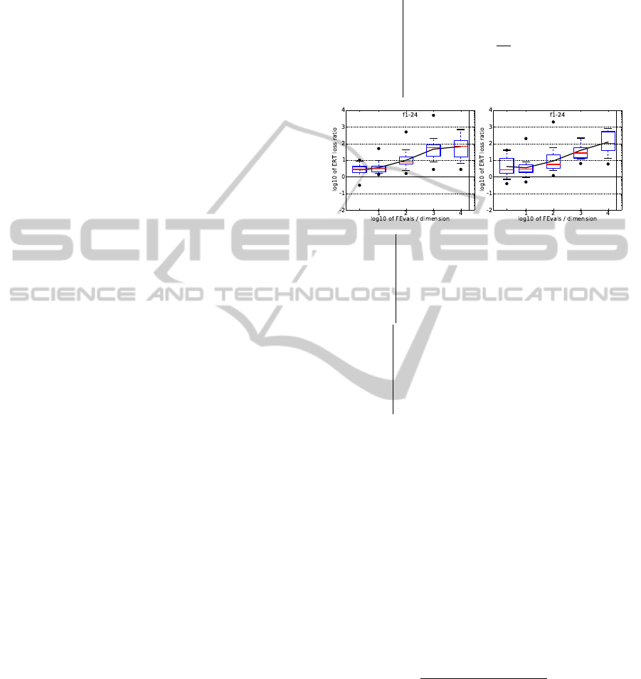
Figure 2: The CMSA-shr-ES. ERT loss ratio (in number

of f -evaluations divided by dimension) divided by the best

ERT seen in GECCO-BBOB-2009 for the target f

, or, if

the best algorithm reached a better target within the budget,

the budget divided by the best ERT. Line: geometric mean.

Box-Whisker error bar: 25-75%-ile with median (box), 10-

90%-ile (caps), and minimum and maximum ERT loss ra-

tio (points). The vertical line gives the maximal number of

function evaluations in a single trial in this function subset.

ning time (ERT) gives the expected value of the func-

tion evaluations ( f -evaluations) the algorithm needs

to reach the target value with the required precision

for the ﬁrst time, see (Hansen et al., 2012). In this

paper, we use

ERT =

#(FEs( f

best

≥ f

target

))

#succ

(28)

as an estimate by summing up the ﬁtness evaluations

FEs( f

best

≥ f

target

) of each run until the ﬁtness of the

best individual is smaller than the target value, di-

vided by all successfull runs.

AdaptingtheCovarianceMatrixinEvolutionStrategies

5-D 20-D

–f

in 5-D, maxFE/D=20000

#FEs/D best 10% 25% med 75% 90%

2 0.33 0.78 1.6 2.5 3.9 7.1

10 1.1 1.5 2.0 2.8 4.6 18

100 1.5 2.5 4.3 6.8 15 57

1e3 2.7 6.9 15 34 75 5.7e2

1e4 2.7 8.0 12 84 4.7e2 7.1e2

1e5 2.7 8.0 12 68 5.9e2 1.2e3

/D 2e4 2e4 2e4 2e4 2e4 2e4

–f

in 20-D, maxFE/D=20000

#FEs/D best 10% 25% med 75% 90%

2 0.23 0.73 1.6 2.3 13 40

10 0.45 0.75 1.4 2.8 4.6 27

100 1.9 2.4 3.9 8.1 21 59

1e3 6.3 7.2 15 35 81 2.4e2

1e4 5.1 12 40 1.5e2 5.0e2 8.1e2

1e5 5.1 12 52 3.8e2 8.6e2 6.7e3

/D 2e4 2e4 2e4 2e4 2e4 2e4

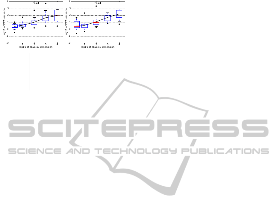
Figure 3: The CMSA-ES. ERT loss ratio (in number of

f -evaluations divided by dimension) divided by the best

ERT seen in GECCO-BBOB-2009 for the target f

, or, if

the best algorithm reached a better target within the budget,

the budget divided by the best ERT. Line: geometric mean.

Box-Whisker error bar: 25-75%-ile with median (box), 10-

90%-ile (caps), and minimum and maximum ERT loss ra-

tio (points). The vertical line gives the maximal number of

function evaluations in a single trial in this function subset.

4.3 Results and Discussion

Due to space restrictions, Figure 4 and Tables 2-3

show only the results from the best experiments which

were achieved for the variant which used (26) together

with (23) as the transformation matrix (called CMSA-

shr-ES in the following). First of all, it should be

noted that there is no signiﬁcant advantage to either

algorithm for the test suite functions. Tables 2 and 3

show the ERT loss ratio with respect to the best re-

sult from the BBOB 2009 workshop for predeﬁned

budgets given in the ﬁrst column. The median per-

formance of both algorithms improves with the di-

mension until the budget of 10

– which is interest-

ing. An increase of the budget goes along with a de-

creased performance which is less pronounced for the

CMSA-shr-ES in the case of the larger dimensional

space. This indicates that the CMSA-shr-ES may per-

form more favorable in larger search spaces as envi-

sioned. Further experiments which a larger maximal

number of ﬁtness evaluations and larger dimensional

spaces will be conducted which should shed more

light on the behavior. Furthermore, the decrease in

performance with the budget hints at a search stagna-

tion probably due to convergence into local optima.

Restart strategies may be beneﬁcial, but since they

have to be ﬁtted to the algorithms, we do not apply

them in the present paper.

Figure 4 shows the expected running time for

reaching the precision of 10

−8

for all 24 functions and

search space dimensionalities. In the case of the sep-

arable functions (1-5), both algorithms show a very

similar behavior, succeeding in optimizing the ﬁrst

two functions and exhibiting difﬁculties in the case

of the difﬁcult rastrigin variants. On the linear slope,

the original CMSA-ES shows fewer expected func-

tion evaluations for smaller dimensions which starts

to change when the dimensionality is increased. For

the functions with ids 6-9, with moderate condition

numbers, there are advantages to the CMSA-shr-ES,

with the exception of the rotated rosenbrock (9). Most

of the functions with high conditioning, ids 10-12,

and 14, can be solved by both variants with slightly

better results for the CMSA-ES. The sharp ridge (id

13) appears as problematic, with the CMSA-shr-ES

showing fewer ﬁtness evaluations for hitting the vari-

ous precisions goals in Table 2.

Interestingly, the CMSA-shr variant seems to per-

form better for the difﬁcult multimodal functions,

e.g., Gallaghers 101 peak function, a ﬁnding which

should be explored in more detail. The results for

the last two multimodal functions can be explained

in part in that the computing resources were insufﬁ-

cient for the optimization. Even the best performing

algorithms from the BBOB workshop needed more

resources than we used in our experiments.

Further experiments will be conducted in order to

shed more light on the behavior. Special attention will

be given to the choice of the shrinkage factor, since

(15) is unlikely to be optimal and may have inﬂu-

enced the outcome strongly. Furthermore, the ques-

tion remains whether the population size should be

increased for the self-adaptation process. Also, larger

search space dimensionalities than N = 20 are of in-

terest.

5 CONCLUSIONS

Evolution strategies are well performing variants of

evolutionary algorithms used in continuous optimiza-

tion. They ultilize normally distributed mutations as

their main search procedure. Their performance de-

pends on the control of the mutation process which is

governed by adapting step-sizes and covariance ma-

trices. One possible improvement concerns the co-

variance matrix adaptation which makes use of the

sample covariance matrix. In statistical research, this

estimate has been identiﬁed as not agreeing well with

the true covariance for the case of large dimensional

ICORES2014-InternationalConferenceonOperationsResearchandEnterpriseSystems

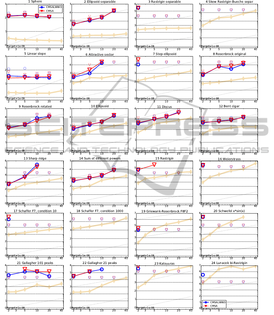
Figure 4: Expected running time (ERT in number of f -evaluations) divided by dimension for target function value 10

−8

log

values versus dimension. Different symbols correspond to different algorithms given in the legend of f

and f

. Light

symbols give the maximum number of function evaluations from the longest trial divided by dimension. Horizontal lines give

linear scaling, slanted dotted lines give quadratic scaling. Black stars indicate statistically better result compared to all other

algorithms with p < 0.01 and Bonferroni correction number of dimensions (six). Legend: .

spaces and small sample sizes, or more correctly for

sample sizes that do not increase sufﬁciently fast with

the dimensionality.

While modern approaches for covariance matrix

adaptation correct the estimate, the question arises

whether the performance of these evolutionary algo-

AdaptingtheCovarianceMatrixinEvolutionStrategies

Table 2: ERT in number of function evaluations divided by the best ERT measured during BBOB-2009 given in the respective

ﬁrst row with the central 80% range divided by two in brackets for different ∆ f values. #succ is the number of trials that

reached the ﬁnal target f

opt

+ 10

−8

. 1:CMSA-S is CMSA-shr-ES and 2:CMSA is CMSA-ES. Bold entries are statistically

signiﬁcantly better compared to the other algorithm, with p = 0.05 or p = 10

−k

where k ∈{2,3,4, ... }is the number following

the ? symbol, with Bonferroni correction of 48. A ↓ indicates the same tested against the best BBOB-2009.

5-D 20-D

∆ f 1e+1 1e-1 1e-3 1e-5 1e-7 #succ

11 12 12 12 12 15/15

1: CMSA-S 2.4(2) 12(4) 25(6) 38(8) 53(8) 15/15

2: CMSA 2.4(2) 12(4) 26(7) 40(8) 54(15) 15/15

83 88 90 92 94 15/15

1: CMSA-S 26(21) 44(24) 53(30) 56(30) 57(29) 15/15

2: CMSA 19(15) 47(19) 54(23) 60(23) 63(30) 15/15

716 1637 1646 1650 1654 15/15

1: CMSA-S 22(70) ∞ ∞ ∞ ∞1.0e5 0/15

2: CMSA 94(140) ∞ ∞ ∞ ∞1.0e5 0/15

809 1688 1817 1886 1903 15/15

1: CMSA-S 46(62) ∞ ∞ ∞ ∞1.0e5 0/15

2: CMSA 186(247) ∞ ∞ ∞ ∞1.0e5 0/15

10 10 10 10 10 15/15

1: CMSA-S 8.6(3) 16(6) 17(6) 17(6) 17(6) 15/15

2: CMSA 8.2(3) 13(6) 14(6) 14(6) 14(6) 15/15

114 281 580 1038 1332 15/15

1: CMSA-S 2.0(1.0) 2.6(1.0) 3.2(3) 2.5(1) 3.2(3) 15/15

2: CMSA 1.6(0.9) 2.2(0.9) 3.2(3) 3.7(3) 5.8(4) 15/15

24 1171 1572 1572 1597 15/15

1: CMSA-S 57(5) 1217(1281) ∞ ∞ ∞1.0e5 0/15

2: CMSA 123(3) ∞ ∞ ∞ ∞1.0e5 0/15

73 336 391 410 422 15/15

1: CMSA-S 2.6(1) 88(152) 79(133) 76(125) 75(122) 12/15

2: CMSA 3.0(1) 85(151) 77(131) 74(124) 72(122) 12/15

35 214 300 335 369 15/15

1: CMSA-S 2.7(2) 15(9) 15(8) 15(7) 15(7) 15/15

2: CMSA 2.9(1) 17(9) 16(7) 16(7) 15(7) 15/15

349 574 626 829 880 15/15

1: CMSA-S 6.7(6) 6.7(5) 7.6(5) 6.3(4) 6.3(3) 15/15

2: CMSA 7.2(4) 7.4(5) 8.3(5) 7.3(5) 7.4(4) 15/15

143 763 1177 1467 1673 15/15

1: CMSA-S 8.8(8) 4.7(2) 3.5(2) 3.1(1) 2.9(1) 15/15

2: CMSA 7.3(6) 4.0(3) 3.3(2) 3.0(2) 2.8(1) 15/15

108 371 461 1303 1494 15/15

1: CMSA-S

14(17) 20(22) 22(19) 10(9) 11(9) 15/15

2: CMSA 9.1(2) 17(21) 19(18) 9.4(9) 10(8) 15/15

132 250 1310 1752 2255 15/15

1: CMSA-S 12(13) 25(16) 7.1(4) 8.2(3) 13(16) 14/15

2: CMSA 5.0(7) 27(25) 7.2(5) 7.2(4) 7.0(3) 14/15

10 58 139 251 476 15/15

1: CMSA-S 1.6(2) 2.9(1) 5.7(2) 8.6(3) 8.1(4) 15/15

2: CMSA 1.3(2) 3.4(1) 5.4(2) 8.7(4) 8.3(4) 15/15

511 19369 20073 20769 21359 14/15

1: CMSA-S 15(1) ∞ ∞ ∞ ∞1.0e5 0/15

2: CMSA 132(196) 72(80) 70(77) 68(77) 66(77) 1/15

120 2662 10449 11644 12095 15/15

1: CMSA-S 3.1(3) 526(620) ∞ ∞ ∞1.0e5 0/15

2: CMSA 3.3(3) 245(282) ∞ ∞ ∞1.0e5 0/15

5.2 899 3669 6351 7934 15/15

1: CMSA-S 3.3(5) 98(167) ∞ ∞ ∞1.0e5 0/15

2: CMSA 2.6(3) 223(278) 177(218) ∞ ∞1.0e5 0/15

103 3968 9280 10905 12469 15/15

1: CMSA-S 70(0.7) 101(126) ∞ ∞ ∞1.0e5 0/15

2: CMSA 0.90(0.7) 22(38) 151(172) ∞ ∞1.0e5 0/15

1 242 1.2e5 1.2e5 1.2e5 15/15

1: CMSA-S 3.1(2) 2730(3097) ∞ ∞ ∞1.0e5 0/15

2: CMSA 3.0(3) 1186(1448) ∞ ∞ ∞1.0e5 0/15

16 38111 54470 54861 55313 14/15

1: CMSA-S 1.6(1) ∞ ∞ ∞ ∞1.0e5 0/15

2: CMSA 1.9(1) ∞ ∞ ∞ ∞1.0e5 0/15

41 1674 1705 1729 1757 14/15

1: CMSA-S377(1220) 388(448) 382(469)376(434)370(455) 2/15

2: CMSA 612(1220) 836(970) 821(909)810(882)797(939) 1/15

71 938 1008 1040 1068 14/15

1: CMSA-S514(705) 693(853) 645(793)626(673)610(773) 2/15

2: CMSA 513(705) 694(852) 646(794)626(721)610(703) 2/15

3.0 14249 31654 33030 34256 15/15

1: CMSA-S 2.0(2) ∞ ∞ ∞ ∞1.0e5 0/15

2: CMSA 3.2(3) ∞ ∞ ∞ ∞1.0e5 0/15

1622 6.4e6 9.6e6 1.3e7 1.3e7 3/15

1: CMSA-S 33(62) ∞ ∞ ∞ ∞1.0e5 0/15

2: CMSA 17(31) ∞ ∞ ∞ ∞1.0e5 0/15

∆ f 1e+1 1e-1 1e-3 1e-5 1e-7 #succ

43 43 43 43 43 15/15

1: CMSA-S 4.7(1) 15(3) 27(3) 38(2) 48(3) 15/15

2: CMSA 4.7(0.9) 14(2) 24(2) 35(3) 46(3) 15/15

385 387 390 391 393 15/15

1: CMSA-S331(232) 567(121) 647(81) 704(91) 755(82) 15/15

2: CMSA 332(106) 561(127) 637(154) 687(182)786(186) 14/15

5066 7635 7643 7646 7651 15/15

1: CMSA-S ∞ ∞ ∞ ∞ ∞4.0e5 0/15

2: CMSA ∞ ∞ ∞ ∞ ∞4.0e5 0/15

4722 7666 7700 7758 1.4e5 9/15

1: CMSA-S ∞ ∞ ∞ ∞ ∞4.0e5 0/15

2: CMSA ∞ ∞ ∞ ∞ ∞4.0e5 0/15

41 41 41 41 41 15/15

1: CMSA-S 10(3) 13(4) 13(4) 13(4) 13(4) 15/15

2: CMSA 11(3) 16(4) 16(4) 16(4) 16(4) 15/15

1296 3413 5220 6728 8409 15/15

1: CMSA-S 1.6(1) 6.4(10) 63(78) 388(475)682(690) 0/15

2: CMSA 1.7(0.4) 7.0(6) 231(278) ∞ ∞4.0e5 0/15

1351 9503 16524 16524 16969 15/15

1: CMSA-S649(862) ∞ ∞ ∞ ∞4.0e5 0/15

2: CMSA 299(444) ∞ ∞ ∞ ∞4.0e5 0/15

2039 4040 4219 4371 4484 15/15

1: CMSA-S 25(9) 49(50) 50(47) 50(49) 50(51) 13/15

2: CMSA 23(14) 67(62) 67(60) 66(58) 66(57) 11/15

1716 3277 3455 3594 3727 15/15

1: CMSA-S 27(10) 63(64) 64(60) 64(57) 64(54) 13/15

2: CMSA 27(7) 52(8) 54(8) 54(9) 54(8) 14/15

7413 10735 14920 17073 17476 15/15

1: CMSA-S 17(6) 19(5) 15(4) 15(3) 15(3) 15/15

2: CMSA 17(10) 21(5) 17(5) 16(5) 18(5) 14/15

1002 6278 9762 12285 14831 15/15

1: CMSA-S 14(4) 4.1(1) 4.2(1) 5.1(3) 5.5(3) 15/15

2: CMSA 13(5) 3.6(1) 3.8(1.0) 4.6(2) 4.8(1) 15/15

1042 2740 4140 12407 13827 15/15

1: CMSA-S

8.5(16) 23(22) 26(15) 12(5) 12(4) 15/15

2: CMSA 5.8(15) 23(25) 26(16) 12(6) 13(6) 15/15

652 2751 18749 24455 30201 15/15

1: CMSA-S 46(0.8) 583(727) 299(325) ∞ ∞4.0e5 0/15

2: CMSA 704(921) 946(1163) ∞ ∞ ∞4.0e5 0/15

75 304 932 1648 15661 15/15

1: CMSA-S 2.0(0.6) 2.6(0.5) 5.9(2) 16(5) 6.8(2) 14/15

2: CMSA 2.0(0.6) 2.6(0.7) 6.2(0.8) 16(5) 6.0(2) 15/15

30378 3.1e5 3.2e5 4.5e5 4.6e5 15/15

1: CMSA-S ∞ ∞ ∞ ∞ ∞4.0e5 0/15

2: CMSA ∞ ∞ ∞ ∞ ∞4.0e5 0/15

1384 77015 1.9e5 2.0e5 2.2e5 15/15

1: CMSA-S 2.9(3) ∞ ∞ ∞ ∞4.0e5 0/15

2: CMSA 107(146) ∞ ∞ ∞ ∞4.0e5 0/15

63 4005 30677 56288 80472 15/15

1: CMSA-S 1.1(1) 1399(1498) ∞ ∞ ∞4.0e5 0/15

2: CMSA 1.1(1) 650(749) ∞ ∞ ∞4.0e5 0/15

621 19561 67569 1.3e5 1.5e5 15/15

1: CMSA-S 0.96(0.5) ∞ ∞ ∞ ∞4.0e5 0/15

2: CMSA 1.0(0.4) ∞ ∞ ∞ ∞4.0e5 0/15

1 3.4e5 6.2e6 6.7e6 6.7e6 15/15

1: CMSA-S 4.8(4) ∞ ∞ ∞ ∞4.0e5 0/15

2: CMSA 6.4(9) ∞ ∞ ∞ ∞4.0e5 0/15

82 3.1e6 5.5e6 5.6e6 5.6e6 14/15

1: CMSA-S 2.0(0.6) ∞ ∞ ∞ ∞4.0e5 0/15

2: CMSA 2.0(0.9) ∞ ∞ ∞ ∞4.0e5 0/15

561 14103 14643 15567 17589 15/15

1: CMSA-S 51(1.0) 43(57) 41(55) 39(51) 34(45) 6/15

2: CMSA 179(356) 184(227) 178(191) 167(193)148(171) 2/15

467 23491 24948 26847 1.3e5 12/15

1: CMSA-S430(857) ∞ ∞ ∞ ∞4.0e5 0/15

2: CMSA 429(857) ∞ ∞ ∞ ∞4.0e5 0/15

3.2 67457 4.9e5 8.1e5 8.4e5 15/15

1: CMSA-S 2.1(2) ∞ ∞ ∞ ∞4.0e5 0/15

2: CMSA 2.3(3) ∞ ∞ ∞ ∞4.0e5 0/15

1.3e6 5.2e7 5.2e7 5.2e7 5.2e7 3/15

1: CMSA-S ∞ ∞ ∞ ∞ ∞4.0e5 0/15

2: CMSA ∞ ∞ ∞ ∞ ∞4.0e5 0/15

rithms may be further improved by applying other es-

timators for the covariance.

This paper considered a combination of two es-

timation approaches to provide a ﬁrst step on this

ICORES2014-InternationalConferenceonOperationsResearchandEnterpriseSystems

way. Shrinkage estimators shrink the sample covari-

ance matrix towards the identity matrix or diagonal

matrix in the case of the paper. In cases, where the

ﬁtness function requires highly different eigenvalues

and a rotation other than the cartesian coordinate sys-

tem this may be problematic. Therefore, a switch to-

wards the eigenspace of the covariance matrix was

proposed in this paper and investigated in experiments

on the BBOB test suite.

REFERENCES

Audet, C. (2013). A survey on direct search methods

for blackbox optimization and their applications. In

Mathematics without boundaries: Surveys in inter-

disciplinary research. Springer. To appear. Also Les

Cahiers du GERAD G-2012-53, 2012.

Bai, Z. D. and Silverstein, J. W. (1998). No eigenvalues

outside the support of the limiting spectral distribution

of large-dimensional sample covariance matrices. The

Annals of Probability, 26(1):316–345.

Beyer, H.-G. (2001). The Theory of Evolution Strategies.

Natural Computing Series. Springer, Heidelberg.

Beyer, H.-G. and Meyer-Nieberg, S. (2006). Self-adaptation

of evolution strategies under noisy ﬁtness evalua-

tions. Genetic Programming and Evolvable Machines,

7(4):295–328.

Beyer, H.-G. and Schwefel, H.-P. (2002). Evolution strate-

gies: A comprehensive introduction. Natural Com-

puting, 1(1):3–52.

Beyer, H.-G. and Sendhoff, B. (2008). Covariance matrix

adaptation revisited - the CMSA evolution strategy -.

In Rudolph, G. et al., editors, PPSN, volume 5199 of

Lecture Notes in Computer Science, pages 123–132.

Springer.

Chen, X., Wang, Z., and McKeown, M. (2012). Shrinkage-

to-tapering estimation of large covariance matri-

ces. Signal Processing, IEEE Transactions on,

60(11):5640–5656.

Chen, Y., Wiesel, A., Eldar, Y. C., and Hero, A. O.

(2010). Shrinkage algorithms for MMSE covariance

estimation. IEEE Transactions on Signal Processing,

58(10):5016–5029.

Conn, A. R., Scheinberg, K., and Vicente, L. N. (2009).

Introduction to Derivative-Free Optimization. MOS-

SIAM Series on Optimization. SIAM.

Dong, W. and Yao, X. (2007). Covariance matrix repair-

ing in gaussian based EDAs. In Evolutionary Com-

putation, 2007. CEC 2007. IEEE Congress on, pages

415–422.

Eiben, A. E. and Smith, J. E. (2003). Introduction to

Evolutionary Computing. Natural Computing Series.

Springer, Berlin.

Finck, S., Hansen, N., Ros, R., and Auger, A. (2010).

Real-parameter black-box optimization benchmark-

ing 2010: Presentation of the noiseless functions.

Technical report, Institute National de Recherche en

Informatique et Automatique. 2009/22.

Fisher, T. J. and Sun, X. (2011). Improved Stein-type

shrinkage estimators for the high-dimensional mul-

tivariate normal covariance matrix. Computational

Statistics & Data Analysis, 55(5):1909 – 1918.

Hansen, N. (2006). The CMA evolution strategy: A com-

paring review. In Lozano, J. et al., editors, To-

wards a new evolutionary computation. Advances in

estimation of distribution algorithms, pages 75–102.

Springer.

Hansen, N., Auger, A., Finck, S., and Ros, R. (2012).

Real-parameter black-box optimization benchmark-

ing 2012: Experimental setup. Technical report, IN-

RIA.

Hansen, N., Auger, A., Ros, R., Finck, S., and Po

ık, P.

(2010). Comparing results of 31 algorithms from the

black-box optimization benchmarking BBOB-2009.

In Proceedings of the 12th annual conference com-

panion on Genetic and evolutionary computation,

GECCO ’10, pages 1689–1696, New York, NY, USA.

ACM.

Hansen, N. and Ostermeier, A. (2001). Completely deran-

domized self-adaptation in evolution strategies. Evo-

lutionary Computation, 9(2):159–195.

Huber, P. J. (1981). Robust Statistics. Wiley, New York.

Ledoit, O. and Wolf, M. (2004). A well-conditioned estima-

tor for large dimensional covariance matrices. Journal

of Multivariate Analysis Archive, 88(2):265–411.

Ledoit, O. and Wolf, M. (2012). Non-linear shrinkage esti-

mation of large dimensional covariance matrices. The

Annals of Statistics, 40(2):1024–1060.

Meyer-Nieberg, S. and Beyer, H.-G. (2007). Self-adaptation

in evolutionary algorithms. In Lobo, F., Lima, C., and

Michalewicz, Z., editors, Parameter Setting in Evo-

lutionary Algorithms, pages 47–76. Springer Verlag,

Heidelberg.

Rechenberg, I. (1973). Evolutionsstrategie: Optimierung

technischer Systeme nach Prinzipien der biologischen

Evolution. Frommann-Holzboog Verlag, Stuttgart.

Sch

affer, J. and Strimmer, K. (2005). A shrinkage approach

to large-scale covariance matrix estimation and impli-

cations for functional genomics,. Statistical Applica-

tions in Genetics and Molecular Biology, 4(1):Article

32.

Schwefel, H.-P. (1981). Numerical Optimization of Com-

puter Models. Wiley, Chichester.

Stein, C. (1956). Inadmissibility of the usual estimator for

the mean of a multivariate distribution. In Proc. 3rd

Berkeley Symp. Math. Statist. Prob. 1, pages 197–206.

Berkeley, CA.

Stein, C. (1975). Estimation of a covariance matrix. In Rietz

Lecture, 39th Annual Meeting. IMS, Atlanta, GA.

Thomaz, C. E., Gillies, D., and Feitosa, R. (2004). A new

covariance estimate for bayesian classiﬁers in biomet-

ric recognition. Circuits and Systems for Video Tech-

nology, IEEE Transactions on, 14(2):214–223.

AdaptingtheCovarianceMatrixinEvolutionStrategies