
The p-Median Problem with Concave Costs
Chuan Xu
1
, Abdel Lisser
1
, Janny Leung
2
and Marc Letournel
1
1
Laboratoire de Recherche en Informatique(LRI),B ˆat 650, Universit
´
e Paris-Sud,
91405, Orsay Cedex, France
2
Department of Systems Engineering and Engineering Management,
The Chinese University of Hong Kong, Hong Kong, Hong Kong
Keywords:
Nonlinear Integer Programming, p-Median, Concave Cost, Linearization, VNS.
Abstract:
In this paper, we propose a capacitated p-median problem with concave costs, in which the global cost incurred
for each established facility is a concave function of the quantity q delivered by this facility. We use DICOPT
to solve this concave model. And then we transform this model into a linear programming problem and solve it
using the commercial solver CPLEX. We also use the metaheuristic Variable Neighbourhood Search (VNS) to
solve this problem. Computational results show that our linearization method helps to improve the calculations
of the concave model. With VNS, we solve large size instances with up to 1500 facilities within a reasonable
CPU time.
1 INTRODUCTION
The p-median problem has been widely studied in the
literature during the last decades especially its linear
version. In this paper, we study and solve large size
instances using particular linearization of the concave
function in order to solve the problem with LP soft-
ware packages. We also study an efficient implemen-
tation of VNS to solve large size instances.
Given a set of n facility sites and m demand cus-
tomers, the p-median problem (PMP) selects exactly
p sites at minimum distribution costs between the cus-
tomers and their open facilities. The PMP was for-
mulated as a zero-one programming problem in 1970
(ReVelle and Swain, 1970). Later, it was proven to
be a NP-hard (Kariv and Hakimi, 1979). The capac-
itated p-median problem (CPMP) is an extension of
the PMP which considers capacities for the service to
be given by each site, i.e., the total service demanded
by customers cannot exceed its service capacities. It
also arises in other contexts like those of vehicle rout-
ing, network design, political districting.
To solve large PMP, Avella et al. (2007) pre-
sented a Branch-Cut-Price algorithm. In (Beltran
et al., 2006), authors introduced a semi-Lagrangian
relaxation to generate lower bounds. Several approx-
imation methods were proposed (Charikar and Guha,
1999; Jain and Vazirani, 2001). Considering to solve
CPMP, heuristics and metaheuristics are the predom-
inant techniques. Ceselli and Righini (2005) pro-
posed a branch and price algorithm. Fleszar and Hindi
(2008) applied an effective VNS to CPMP. Others like
scatter search heuristic (Xu et al., 2010), genetic algo-
rithm (Stanimirovi
´
c, 2008) were also applied to solve
this problem. Recently, some hybrid heuristics ap-
proaches were developed to enhance the performance
like (Landa-Torres et al., 2012; Yaghini et al., 2013).
Both the CPMP and the PMP aforementioned can
be formulated as linear integer programming prob-
lems. In our model, the CPMP problem with con-
cave cost means that the distribution cost of each fa-
cility site depends on the total quantity delivered by
the site. The unit distribution cost decreases with
the increased quantity of output or demand generating
economy of scales. This variant is in the class of non-
linear location problem. The objective function of our
model is the same as the model proposed by Dupont
(2008). In his work, he studied a concave facility lo-
cation problem without capacity constraint and solved
it with a branch and bound algorithm. There are also
many other models using concave functions, see for
instances (Nagy and Salhi, 2007; Ghoseiri and Ghan-
nadpour, 2007). Sun and Gu (2002) proposed a net-
work design problem where the function of delivery
cost is concave. Their method consists in omitting
the nonlinear factor and adjusting the solution to ob-
tain an overall approximated optimal solution. Verter
and Dasci (2002) solved the uncapacitated plant lo-
cation and flexible technology acquisition problem
with the monotone increasing concave function. They
205
Xu C., Lisser A., Leung J. and Letournel M..
The p-Median Problem with Concave Costs.
DOI: 10.5220/0004832502050212
In Proceedings of the 3rd International Conference on Operations Research and Enterprise Systems (ICORES-2014), pages 205-212
ISBN: 978-989-758-017-8
Copyright
c
2014 SCITEPRESS (Science and Technology Publications, Lda.)

adopted the progressive piecewise linear underestima-
tion (PPLU) technique (Verter and Dincer, 1995) to
simplify the model.
In our case, we adopt PPLU method to linearize
the objective function. Then, since the model is con-
verted into an integer program, we apply the VNS to
solve it.
VNS was first proposed by Hansen and Mladen-
ovi
´
c (1997) and rapidly developed since then. It has
been applied to the design problems in communica-
tion, location problems, data mining, knapsack and
packing problems. For more details on VNS and its
main applications to p-median problem, see (Hansen
et al., 2010; Fathali and Kakhki, 2006; Osman and
Ahmadi, 2006; Hansen et al., 2009).
This paper is structured as follows. Section 2 in-
troduces a mathematical formulation of the problem.
Section 3 presents solution methods. Section 4 shows
and discusses the computational results. We conclude
the paper in Section 5.
2 MATHEMATICAL
FORMULATION
Our model is a capacitated p-median problem with
concave distribution costs. We assume that our dis-
tribution costs are concave functions of the quantity
q delivered by the facility site which is a situation in
economies of scale. The main difference between our
model and the standard model of CPMP is that, in-
stead of minimizing the distribution costs related to
the distances between sites and customers, we stud-
ied an objective function of distribution costs related
to q and introduced a distribution range R for each
facility site to constrain distances between sites and
customers.
In practice, distribution costs are not always
dependent on the distance between sites and cus-
tomers but on the total quantity delivered by the sites
(Dupont, 2008). For instance, if we outsource our
transportation service to a third party logistics (3PL),
the cost will be related to the quantity that we ask 3PL
to deliver. That’s the linear part B
i
·q
i
included in our
objective function. And the more we delivered, the
less we pay for the unit distribution cost. The square
root of q
i
in our objective function follows this rule.
The aim of our model is to select a subset of po-
tential sites to satisfy all the customers requirements
at minimum distribution costs.
We use the following notation in our model:
Let I = {1,...,n} be a set of sites, J = {1,...,m} be a
set of customers. I( j) shows the set of sites that can
deliver customer j. J(i) shows the set of customers
that can be delivered by site i. I( j),J(i) can be ob-
tained by comparing the distance between site i and
customer j with their distribution range R
i
,R
j
. d
j
is
the demand of customer j. p is the median parame-
ter. δ
i
presents the maximum capacity of site i. F
i
(q
i
)
presents the concave function for each site i which has
A
i
,B
i
,C
i
as coefficients.
We consider three decision variables:
z
i j
: the quantity delivered by site i to customer j,
q
i
: the quantity delivered by site i,
y
i
: if site i is open y
i
= 1 otherwise y
i
= 0
The p-median concave costs problem can be writ-
ten as follows:
min
i=n
∑
i=0
F
i
(q
i
) =
i=n
∑
i=0
(A
i
+ B
i
·q
i
+C
i
√
q
i
) ·y
i
(1)
∑
j∈J(i)
z
i j
= q
i
∀i ∈ I, (2)
∑
i∈I( j)
z
i j
= d
j
∀j ∈ J, (3)
∑
i∈I
y
i
= p, (4)
q
i
≤ δ
i
y
i
∀i ∈ I, (5)
y
i
∈ {0,1} ∀i ∈ I, (6)
q
i
≥ 0 ∀i ∈ I,
z
i j
≥ 0 ∀i ∈ I, j ∈J.
The objective function (1) minimizes the concave
distribution costs. Constraint (2) shows that the quan-
tity delivered by site i is the sum of all the customers’
demands for this site. Constraint (3) shows that every
customer’s request must be satisfied. Constraint (4)
presents the number of sites to open. Constraint (5)
gives the capacity of each site. Constraint (6) defines
variables domain.
3 SOLUTION METHODS
We use two different methods to solve the p-median
problem (1-6) i.e., a linear program obtained by lin-
earizing the concave function and the metaheuristic
VNS.
3.1 Linearization Method
We linearize the function F
i
(q
i
) = A
i
+B
i
·q
i
+C
i
√
q
i
by dividing the range of each site capacity into small
intervals. We assume that the range of the site i is
[γ
i
,δ
i
].
Then, we obtain a set of small intervals i.e.,
{[γ
i
0
,γ
i
1
],[γ
i
1
,γ
i
2
],... ,[γ
i
K−1
,γ
i
K
]} with γ
i
0
= γ
i
,γ
i
K
=
ICORES2014-InternationalConferenceonOperationsResearchandEnterpriseSystems
206

δi. Therefore, the linear function in the kth interval
[γ
i
k−1
,γ
ik
] is:
f
i
k
(q
i
) = λ
i
k
q
i
+ β
i
k
. (7)
λ
i
k
=
F
i
(γ
i
k
) −F
i
(γ
i
k−1
)
γ
i
k
−γ
i
k−1
. (8)
β
i
k
=
γ
i
k
F
i
(γ
i
k−1
) −γ
i
k
−1
F
i
(γ
i
k
)
γ
i
k
−γ
i
k−1
. (9)
where K is the number of intervals. If K is large, the
approximation of the concave function is sharp.
From the formulas aforementioned, we can obtain
the values of λ
i
k
and β
i
k
with the boundary of the kth
interval and the coefficients A
i
,B
i
,C
i
in the concave
function F
i
(q
i
). In order to figure out the boundary
values γ
i
k−1
and γ
i
k
, we need to compute the number
of intervals K.
q
i
k
=
C
i
2(λ
i
k
−B
i
)
2
. (10)
d
i
k
= F
i
(q
i
k
) − f
i
(q
i
k
) . (11)
ε
i
k
=
d
i
k
F
i
(q
i
k
)
. (12)
where q
i
k
is the point with the greatest gradient in the
concave function which also means the farthest point
from the linear function; d
i
k
represents the farthest
distance and ε
i
k
shows the percentage of deviation be-
tween the concave function and the linear function.
We divide the range of capacity of each site continu-
ously until the value of ε
i
k
reaches the reference value
that we have set before. At the end, we can figure
out the value of K. After the linearization, we use bi-
nary variable y
i
k
to check whether the total request
for site i is in the k
th
interval. If so, y
i
k
= 1 and 0 o.w.
Once the interval is located, the cost function is built
based on suitable values of λ and β. Then, we add
binary variables y
1i
k
,y
2i
k
such that y
i
k
= y
1i
k
·y
2i
k
and
Q
i
k
= q
i
·y
i
k
to perform the linearization of the terms
q
i
y
i
k
. Those binary variables are defined as follows:
y
i
k
= 1 if q
i
∈ (γ
i
k−1
,γ
i
k
], y
1i
k
= 1 if q
i
> γ
i
k
−1
and
y
2i
k
= 1 if q
i
≤ γ
i
k
.
Hence, F
i
(q
i
) can be written as:
F
i
(q
i
) ≈
k=K
∑
k=1
f
i
k
(q
i
)y
i
k
=
k=K
∑
k=1
(λ
i
k
q
i
+ β
i
k
)y
i
k
,∀i ∈I.
(13)
Based on the aforementioned linearization, the
equivalent linear programming problem is as follows:
min
i=n
∑
i=0
k=K
∑
k=1
λ
i
k
Q
i
k
+ β
i
k
y
i
k
(14)
s.t.
∑
i∈I( j)
z
i j
= d
j
∀j ∈ J, (15)
∑
j∈J(i)
z
i j
= q
i
∀i ∈ I, (16)
∑
i∈I
y
i
= p ∀i ∈ I, (17)
k=K
∑
k=1
y
i
k
= y
i
∀i ∈ I, (18)
γ
i
y
i
≤ q
i
≤ δ
i
y
i
∀i ∈ I, (19)
q
i
≥ (γ
i
k−1
+ 1)y
1i
k
∀i ∈ I,∀k ∈ [1,K], (20)
q
i
≤ γ
i
k−1
(1 −y
1i
k
) + δ
i
y
1i
k
∀i ∈ I,∀k ∈ [1,K], (21)
q
i
≥ (γ
i
k
+ 1)(1 −y
2i
k
) ∀i ∈ I,∀k ∈[1, K], (22)
q
i
≤ γ
i
k
y
2i
k
+ δ
i
(1 −y
2i
k
) ∀i ∈ I,∀k ∈ [1,K], (23)
y
i
k
≤ y
1i
k
,y
i
k
≤ y
2i
k
∀i ∈ I,∀k ∈ [1,K], (24)
y
i
k
≥ y
1i
k
+ y
2i
k
−1 ∀i ∈ I,∀k ∈[1, K], (25)
Q
i
k
≤ q
i
,Q
i
k
≤ δ
i
y
i
k
∀i ∈ I,∀k ∈ [1,K], (26)
Q
i
k
≥ q
i
−δ
i
(1 −y
i
k
) ∀i ∈ I,∀k ∈[1, K], (27)
y
i
,y
i
k
,y
1i
k
,y
2i
k
∈ {0,1} ∀i ∈I,∀k ∈ [1, K], (28)
z
i j
,Q
i
k
,q
i
≥ 0 ∀i ∈ I,∀j ∈ J,∀k ∈ [1,K]. (29)
There are (14nK + 5n + nm + m + 1) constraints.
Constraints (20-27) are linearization constraints.
Proposition 3.1. The farthest distance between the
concave function F
i
and the linear function f
i
is lo-
cated in the first interval [γ
i0
,γ
i1
] and its value is d
i1
.
Proof. We substitute the part F
i
(q
i
) with the concave
function F
i
(q
i
) = A
i
+ B
i
·q
i
+C
i
√
q
i
in (8) and (9).
Then we obtain the values of λ
i
k
and β
i
k
as follows:
λ
i
k
= B
i
+
C
i
√
γ
i
k
+
√
γ
i
k−1
. (30)
β
i
k
= A
i
+
C
i
√
γ
i
k
γ
i
k−1
(
√
γ
i
k
+
√
γ
i
k−1
)
. (31)
By using (10), we get another function of λ
i
k
in terms
of q
i
k
:
λ
i
k
= B
i
+
C
i
2
√
q
i
k
. (32)
Combining (30) and (32), we obtain
q
i
k
=
(
√
γ
i
k
+
√
γ
i
k−1
)
2
4
. (33)
Equation (33) reveals that the value of q
i
k
has no
relationship with the coefficients A
i
,B
i
and C
i
of the
concave function. It is related to the boundary of the
interval.
Thep-MedianProblemwithConcaveCosts
207

Putting all the formulas aforementioned into (11)
which gives the definition of d
i
k
, we obtain a function
of d
i
k
related to the value of γ
i
k
. Then, we set h =
γ
i
k
−γ
i
k−1
where h is a constant if we know the number
of considered intervals.
d
i
k
(γ
i
k
) =
C
i
h
2
4(
√
γ
i
k
+
p
γ
i
k
−h)
3
. (34)
The value of distance d
i
k
is only related to the in-
terval
γ
i
k−1
,γ
i
k
and the coefficient C
i
in the concave
function. This formula of d
i
k
is a decreasing function
of the value of γ
i
k
. Because the part of the function
in the numerator is a decreasing function and the part
in the denominator is an increasing function with the
value of γ
i
k
. As γ
i
k
represents the value of boundary
for the k
th
interval, the smallest value of boundary γ
i
k
is located in the first interval k = 1, thus the distance
d
i
1
in this interval is the farthest. In other words, when
k increases, the value of d
i
k
decreases.
If we set γ
i
= 0, which means the minimum capac-
ity for site i is zero, then
γ
i
1
= h (35)
d
i
1
=
C
i
4
√
h (36)
Proposition 3.2. The linear function in the first inter-
val [γ
i
0
,γ
i
1
] has the maximum percentage of deviation
ε between the concave function and the linear func-
tion.
Proof. In the proposition (1), we proved that d
i
k
is
a decreasing function of the value of k. For the part
F
i
(q
i
k
) in the denominator, we know that with the in-
crease of k, q
i
k
is larger. And F
i
(q
i
k
) is obviously an
increasing function with the value of q
i
k
, because it is
a concave one. Thus, the function in the denomina-
tor is an increasing function with the value of k. So
we can say that ε
i
k
is a decreasing function with the
value of k. When we choose the first interval which
means that k is the smallest (k = 1), the percentage of
deviation is the largest.
We just need to calculate the percentage of devi-
ation in the first interval to decide whether our lin-
earization meets to the reference gap we set before.
The function of ε
i
k
is under the form:
ε
i
k
=
C
i
h
2
[4A
i
+ 2C
i
(
√
γ
i
k
+
p
γ
i
k
−h) + B
i
(
√
γ
i
k
+
p
γ
i
k
−h)
2
]
×
1
(
√
γ
i
k
+
p
γ
i
k
−h)
3
(37)
If we set γ
i
= 0 and k = 1, we get
ε
i
1
=
C
i
√
h
4A
i
+ 2C
i
√
h + B
i
h
(38)
3.2 Variable Neighbourhood Search
Method
VNS is a recent metaheuristic whose basic idea is to
proceed a systematic change of neighbourhood within
a local search algorithm (Hansen and Mladenovi
´
c,
1997). In our case, we initialised our solution by
distributing the customers to their nearest sites with
respect to their distribution ranges. We suppose at
first that each site is responsible for the same num-
ber of customers. The detail is shown in the proce-
dure InitialSolution below. After this procedure, we
obtain our decision vector y = (y
1
,y
2
,...,y
n
). It fol-
lows that the solution space S for the problem contains
n
p
solutions representing all the combinations of p
sites from n candidates. We consider two solutions
x
1
,x
2
∈ S, the distance between them is the number
of y
i
whose values are different. The neighbourhood
k called (N
k
(x)) is a set that contains all solutions at
a distance k from a solution x. The largest distance
(k
max
) of our model is set to min(p,n − p).
The main idea in our local search is to switch a
customer c from a facility site p
out
to another facil-
ity site p
in
, while reducing the distribution costs. At
the same time, the movement should respect the ca-
pacity constraint. In addition, after the movement, we
should consider one median problem for the serving
area of p
in
, p
out
and figure out the most suitable facil-
ity sites to be opened in these two areas. The local
search stops when there exists no more better move-
ments which improve the value of the objective func-
tion.
For each selected site, we calculate the total de-
mand of its customers, called (DN). The algorithm
for choosing c, p
out
, p
in
at each iteration consists in
picking a move −out site p
out
with a smallest value of
DN and a move −in site p
in
with a largest DN value
from all the selected sites. Then we choose a cus-
tomer c with the largest demand of all the customers
delivered by p
out
. The idea of the algorithm consists
in maximizing the quantity delivered by certain sites.
As a result, the unit distribution cost decreases. The
details of this algorithm are shown in the procedure
OneTimeLocalSearch.
4 NUMERICAL EXPERIMENTS
We test our models on the instances introduced by
Osman and Christofides (1994) which can be down-
ICORES2014-InternationalConferenceonOperationsResearchandEnterpriseSystems
208

Procedure 1: VNS(k
max
,r).
Input: k
max
: maximum neighbourhood size; r:
repeated times
Output: The best solution S
best
that we found
S ← InitialSolution();
for k = 1 to k
max
do repeat r times do
/* Generate a random solution from
N
k
(S) */
S1 ← JumpToNeighbor(S,k);
/* Local search */
S1 ← LocalSearch(S1);
if S1.cost < S.cost then
S ←S1, k ←0;
end
end
Procedure 2: InitialSolution.
Output: The initial solution S
P /* P presents the set of selected
median sites,N presents the set of
all the sites */
Range ← n/p;
For each site i, calculate DS[i], the sum of
distances of its Range nearest customers;
for k = 1 to k = p do
s ← the site with smallest DS value in N;
if Q[s]
1
≤Cap[s]
2
then
/* Q[s] gives the quantity
delivered by site s to its
customers, Cap gives the
capacity value for each site
*/
P ∩{s}, N \{s} ;
Recalculate DS value for all the sites in
N ;
end
else
DS[s] ← ∞
end
end
loaded from OR-library
3
. Set A contains 10 instances
of size n = 50, p = 5 and set B contains 10 instances
of size n = 100, p = 10. The parameters A
i
,B
i
,C
i
are generated by Matlab with normal distributions
A
i
∼N (500,100),B
i
∼N (0.04,0.01),C
i
∼N (10,3)
respectively. The distribution range R varies from 35
to 115. The number of intervals k for linearized model
is 30.
Two models are coded on the General Algebraic
3
http://people.brunel.ac.uk/∼mastjjb/jeb/orlib/pmedcapinfo.html
Procedure 3: LocalSearch(S).
Input: The initial Solution S
Output: The local minimum solution S
0
f lag ←true;
while f lag do
f lag ←OneTimeLocalSearch(S);
end
S
0
← S;
return S
0
;
Procedure 4: OneTimeLocalSearch(S).
Input: The intial solution S
Output: The boolean value which siginifies if
we could find a better solution.
P ← S.p sites , P is a set of p-median sites.;
for each site p
in
∈ P in a descending order by
DN[p
in
], the total demand of its customers do
if DN[p
in
] < Cap[p
in
] then
for each p
out
∈ P in an ascending order
by DN[p
out
] such that p
out
! = p
in
∩
DN[p
out
] < DN[p
in
] do
Suppose C
out
is a set of all
customers delivered by the site p
out
;
for each customer c ∈C
out
, in a
descending order by its demand
D[c] do
if D[c] + DN[p
in
] ≤Cap[p
in
] ∩
Dis(c, pin) ≤ R then
/* Dis:distance
matrix,R:distribution
range */
if Move(c, p
in
, p
out
,S) then
/* In the procedure
of Move, we
give the better
solution to S.
*/
return true;
end
end
end
end
end
end
return false;
Modeling System (GAMS). The computational
experiments are carried out on a INTEL I7 2GHZ
computer with 4G RAM.
We solve our concave model (1-6) using a com-
Thep-MedianProblemwithConcaveCosts
209
Procedure 5: Move(c, p
in
, p
out
,S).
Input: c: the customer to move; p
in
, p
out
: the
delivery base site; S: the original
solution
Output: The boolean value which siginifes if
we put the customer c in the delivery
area of p
in
and the changed solution S
cost ← S.cost();
{C
in
} ← c ∪{C
in
};
{C
out
} ← {C
out
} ;
/* C
out
is a set of customers
delivered by site p
out
, we move
customer c out of the delivery
space of p
in
*/
S
0
← One Median Problem (p
in
,C
in
,S);
/* Choose the site i from {p
in
}∩C
in
to
deliver its customers {p
in
}∩C
in
\i
with a minimum distribution cost
*/
S
0
←One Median Problem (p
out
,C
out
,S
0
);
cost
0
← S
0
.cost();
if cost
0
≤ cost then
S ←S
0
;
return true;
end
else
return false;
end
mercial solver Discrete and Continuous Optimizer
(DICOPT ) which was designed to solve mixed inte-
ger non-linear programming problems (MINLP) with
an outer-approximation algorithm (Kocis and Gross-
mann, 1989). This solver can guarantee the global
optimum if the nonlinear function is convex. How-
ever, since our objective function is concave, it gives
an upper bound for the problem. Inside the configura-
tion of DICOPT , we choose CONOPT (Drud, 1996)
as the NLP solver and CPLEX as the MIP solver.
Then, we solve the linearized model (14-29)
which is a mixed integer linear programming using
CPLEX solver.
Firstly, in our experiments, we test our models
with different distribution range R to see the influence
of R. When R is small, each facility site could only
serves certain number of customers. If R is too small,
we can’t even find a feasible solution. After several
trials on R, we choose to run our tests with R from 35
ensuring at least one feasible solution to 115 so that
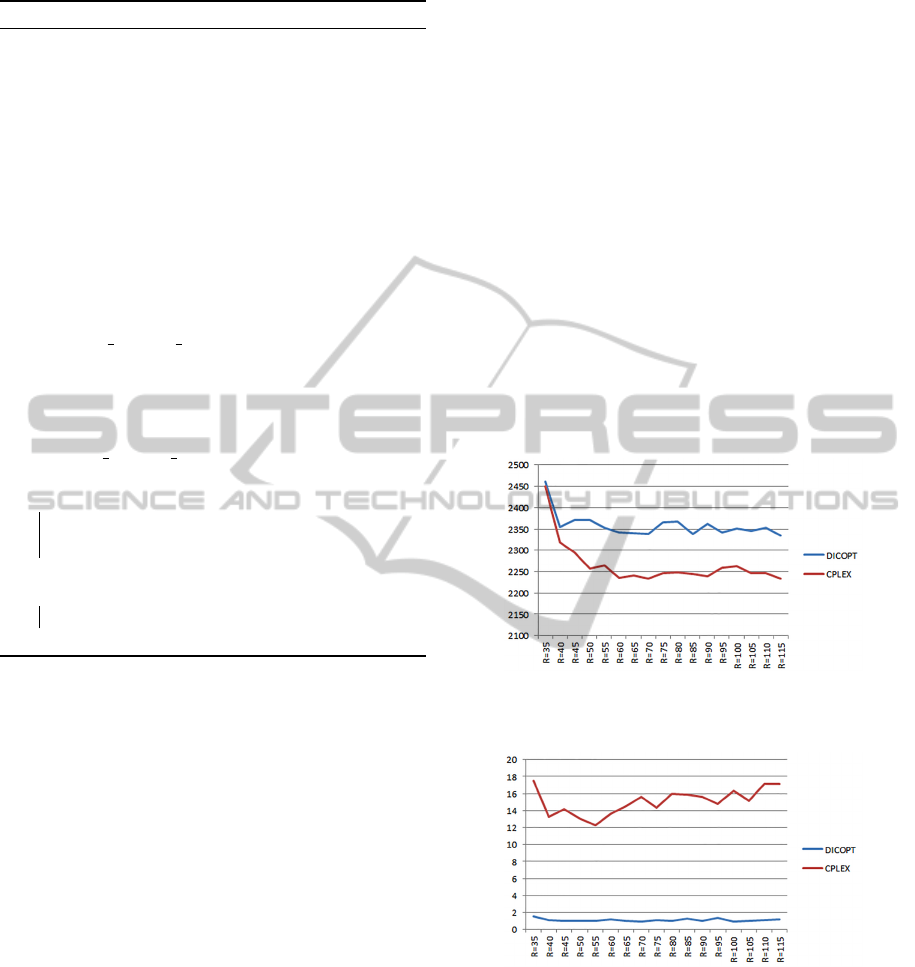
each facility site could serve every customers. Fig.1
shows the average values obtained by DICOPT and
CPLEX for set A instances as the distribution range R
increases. Fig.2 presents the average execution times
of DICOPT and CPLEX in seconds for solving set A
instances. Fig.3 shows the average values obtained by
DICOPT and CPLEX for set B instances.
We can see from Fig.1 that as R increases, we
have more possible choices for sites and customers,
the value of objective function tends to decrease. As
solvers do not always guarantee a global optimal so-
lution, the curves do not decrease smoothly. There
exists some small fluctuations. The values of CPLEX
curve are obtained by solving the linearized model
first with CPELX and then recalculating concave ob-
jective function. Comparing the curve of DICOPT
with the curve of CPLEX, we observed that our lin-
earized model performs better than concave model
in getting global optimal solution using the existing
commercial solvers. Fig.3 shows that our advantage
in quality of solution when solving linearized model
holds also for larger instances of set B.
Figure 1: Average value of solutions of set A instances.
Figure 2: Average execution time of set A instances.
Secondly, we apply our approach of V NS to solve
CPMP with large size instances. The number of sites
is ranging from 100 to 1500. These large instances are
generated randomly following normal distributions.
CPLEX and DICOPT were very time-consuming. In
this case, we only report the lower bounds by solving
linearized model with CPLEX and continue our cal-
culations with V NS. The latter could solve the prob-
lem with up to 1500 sites. The results are presented
in the Tab.1. Columns 1,2,3 give the number of sites,
ICORES2014-InternationalConferenceonOperationsResearchandEnterpriseSystems
210
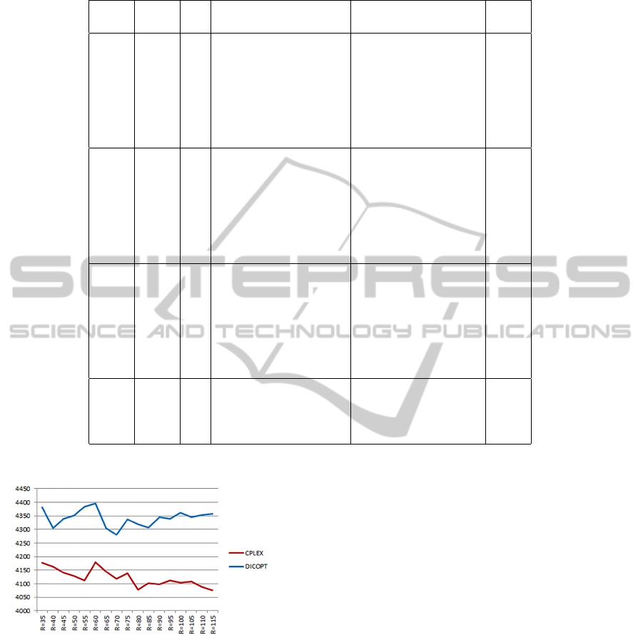
Table 1: Results for the linearized model in the large data; the best solution found in 10 trials of VNS is reported.
CPLEX VNS GAP
N M P Value time Value time %
K
max
=P
50 50 2 26873 132.30 26873 0.11 0.00
60 60 3 31969.2 446.96 31969.2 0.14 0.00
70 70 3 36249.4 289.46 36600.1 0.25 0.01
80 80 3 37362.4 248.90 37362.4 0.24 0.00
90 90 3 43059.8 3341.56 43060.3 0.44 0.00
100 100 3 49056.4 1121.96 49056.4 0.28 0.00
150 150 4 13950
∗
39.51 71413.5 0.18 #
200 200 6 19063.9
∗
67.75 97105.4 3.36 #
250 250 7 24981.6
∗
339.63 118861 10.27 #
300 300 8 30842.6
∗
495.57 137737 22.26 #
350 350 9 80002.1
∗
998.22 162297 50.92 #
400 400 11 47433.5
∗
1637.71 187413 141.40 #
450 450 12 49056.4
∗
1121.96 206303 217.15 #
K
max
=P/3
500 500 13 57710.4
∗
1134.86 227456 195.77 #
600 600 16 83009.0
∗
1535.36 281224 592.29 #
700 700 18 102030.1
∗
1900.24 330264 1018.02 #
800 800 20 142003.5
∗
2503.31 367511 2096.62 #
900 900 23 184030.1
∗
2709.72 430663 1978.83 #
1000 1000 25 240248.2
∗
3501.29 463628 2796.42 #
1200 1200 30 537799 3891.14 #
1300 1300 32 562032 4029.12 #
1400 1400 33 591024 5129.20 #
1500 1500 34 677229 7428.21 #
∗
CPLEX failed to solve the integer problem, only lower bounds values are reported.
Figure 3: Average value of solutions of set B instances.
the number of customers and the median value respec-
tively. Columns 4,5 present the numerical results and
the execution time in seconds for CPLEX and V NS
respectively. Column “GAP” gives the relative gap of
V NS to the optimal solution.
5 CONCLUSIONS
In this paper, we investigate a capacitated p-median
model with concave cost. The cost is a concave func-
tion of the quantity handled by site i. We show that the
problem can be approximated to a mixed linear pro-
gramming problem. An efficient VNS for this model
has been proposed.
We present computational results comparing the
exact formulation and linearized formulation, using
DICOPT,CPLEX respectively. Computational re-
sults show that our linearized method enables to reach
optimal solution of our problem. When using VNS,
we can solve instances with up to 1500 sites. Our
VNS performances show that our adaptation of the
algorithm to this difficult problem is very efficient as
illustrated by the small gaps,i.e. less than 2%.
REFERENCES
Avella, P., Sassano, A., and Vasil’ev, I. (2007). Computa-
tional study of large-scale p-median problems. Math-
ematical Programming, 109(1):89–114.
Beltran, C., Tadonki, C., and Vial, J. P. (2006). Solving
the p-median problem with a semi-lagrangian relax-
Thep-MedianProblemwithConcaveCosts
211

ation. Computational Optimization and Applications,
35(2):239–260.
Ceselli, A. and Righini, G. (2005). A branch-and-price al-
gorithm for the capacitated p-median problem. Net-
works, 45(3):125–142.
Charikar, M. and Guha, S. (1999). Improved combinato-
rial algorithms for the facility location and k-median
problems. In Foundations of Computer Science, 1999.
40th Annual Symposium on, pages 378–388. IEEE.
Drud, A. (1996). Conopt - a system for large scale nonlinear
optimization. REFERENCE MANUAL for CONOPT
Subroutine Library, ARKI Consulting and Develop-
ment A/S.
Dupont, L. (2008). Branch and bound algorithm for a fa-
cility location problem with concave site dependent
costs. International Journal of Production Economics,
112(1):245–254.
Fathali, J. and Kakhki, H. (2006). Solving the p-median
problem with pos/neg weights by variable neighbor-
hood search and some results for special cases. Eu-
ropean journal of operational research, 170(2):440–
462.
Fleszar, K. and Hindi, K. (2008). An effective vns for the
capacitated p-median problem. European Journal of
Operational Research, 191(3):612–622.
Ghoseiri, K. and Ghannadpour, S. (2007). Solving ca-
pacitated p-median problem using genetic algorithm.
In Industrial Engineering and Engineering Manage-
ment, 2007 IEEE International Conference on, pages
885–889. IEEE.
Hansen, P., Brimberg, J., Uro
ˇ
sevi
´
c, D., and Mladenovi
´
c, N.
(2009). Solving large p-median clustering problems
by primal-dual variable neighborhood search. Data
mining and knowledge discovery, 19(3):351–375.
Hansen, P. and Mladenovi
´
c, N. (1997). Variable neigh-
borhood search for the p-median. Location Science,
5(4):207–226.
Hansen, P., Mladenovi
´
c, N., and Moreno P
´
erez, J. (2010).
Variable neighbourhood search: methods and appli-
cations. Annals of Operations Research, 175(1):367–
407.
Jain, K. and Vazirani, V. V. (2001). Approximation algo-
rithms for metric facility location and k-median prob-
lems using the primal-dual schema and lagrangian re-
laxation. Journal of the ACM (JACM), 48(2):274–296.
Kariv, O. and Hakimi, S. (1979). An algorithmic approach
to network location problems. ii: The p-medians.
SIAM Journal on Applied Mathematics, pages 539–
560.
Kocis, G. and Grossmann, I. (1989). Computational ex-
perience with dicopt solving {MINLP} problems in
process systems engineering. Computers & Chemical
Engineering, 13(3):307 – 315.
Landa-Torres, I., Ser, J. D., Salcedo-Sanz, S., Gil-Lopez, S.,
Portilla-Figueras, J., and Alonso-Garrido, O. (2012).
A comparative study of two hybrid grouping evolu-
tionary techniques for the capacitated p-median prob-
lem. Computers & Operations Research, 39(9):2214
– 2222.
Nagy, G. and Salhi, S. (2007). Location-routing: Issues,
models and methods. European Journal of Opera-
tional Research, 177(2):649–672.
Osman, I. and Ahmadi, S. (2006). Guided construction
search metaheuristics for the capacitated p-median
problem with single source constraint. Journal of the
Operational Research Society, 58(1):100–114.
Osman, I. H. and Christofides, N. (1994). Capacitated clus-
tering problems by hybrid simulated annealing and
tabu search. International Transactions in Opera-
tional Research, 1(3):317–336.
ReVelle, C. and Swain, R. (1970). Central facilities loca-
tion. Geographical Analysis, 2(1):30–42.
Stanimirovi
´
c, Z. (2008). A genetic algorithm approach for
the capacitated single allocation p-hub median prob-
lem. Computing and Informatics, 27.
Sun, J. and Gu, Y. (2002). A parametric approach for a
nonlinear discrete location problem. Journal of com-
binatorial optimization, 6(2):119–132.
Verter, V. and Dasci, A. (2002). The plant location and flex-
ible technology acquisition problem. European Jour-
nal of Operational Research, 136(2):366–382.
Verter, V. and Dincer, M. (1995). Facility location and ca-
pacity acquisition: an integrated approach. Naval Re-
search Logistics (NRL), 42(8):1141–1160.
Xu, X., Li, X., Li, X., and Lin, H. (2010). An improved scat-
ter search algorithm for capacitated p-median prob-
lem. In Computer Engineering and Technology (IC-
CET), 2010 2nd International Conference on, vol-
ume 2, pages V2–316. IEEE.
Yaghini, M., Karimi, M., and Rahbar, M. (2013). A hybrid
metaheuristic approach for the capacitated p-median
problem. Applied Soft Computing, 13(9):3922 – 3930.
ICORES2014-InternationalConferenceonOperationsResearchandEnterpriseSystems
212
