
Radio-interferometric Object Trajectory Estimation
Gergely Zachár and Gyula Simon
Department of Computer Science and Systems Technology, University of Pannonia, Veszprém, Hungary
Keywords: Sensor Network, Localization, Tracking, Radio-Interferometry.
Abstract: In this paper a novel radio-interferometric object trajectory estimation method is proposed, which can be
used to track moving objects. The system utilizes a low number of fixed infrastructure nodes equipped with
radio transceivers, and the tracked object also carries a simple transceiver. Selected transmitter
infrastructure nodes produce interference signals at the fixed infrastructure receivers and the tracked
receiver. Transmitter and receiver roles are rotated, thus multiple interference signals are produced, which is
measured by synchronized receiver pairs. Measurements are then compared to pre-computed phase maps
while the object is moving. During object movement the system resolves position ambiguities and the exact
object trajectory is determined. The performance of the proposed method is illustrated by simulation
examples and real measurements.
1 INTRODUCTION
Object localization and object tracking is an
important functionality in many applications and
thus various approaches have been proposed,
including image processing, acoustic, and RF-based
solutions.
Image- and video-based solutions extract
significant visual information from the frames and
thus can find and follow objects along a series of
frames. This approach can be used for object
detection, identification, localization, and tracking,
see e.g. (Comaniciu, 2003). In acoustic ranging
methods the time of flight of acoustic signals
(mainly ultrasound) is measured, and the system
determines pairwise distances between nodes with
known and unknown locations, and from the
pairwise distance set it calculates the unknown
positions, see e.g. (Ajdler, 2004).
Among the RF-based solutions GPS is the most
widespread solution in applications where line of
sight to satellite can be provided. In indoor
applications, however, alternative methods are
searched. Positioning based on signal strength is
probably the simplest of RF-based methods, and can
provide a few meters of accuracy, with sufficiently
dense transmitter infrastructure and an a priori
measured reference map (Au, 2012). Time of flight
of RF signals can also be used for ranging, using a
significantly more sophisticated system (Schwarzer,
2008). To avoid high precision time of flight
measurements, (Maroti, 2005) proposed radio
interferometric measurements and a corresponding
localization method, which can work with
inexpensive hardware and software solutions.
In this paper a novel object tracking method will
be proposed, which utilizes radio-interferometric
measurements. In contrast to the former localization
method of (Maroti, 2005), the proposed solution is
not suitable for localization but for tracking. The
proposed solution is either able to determine the full
track of a moving object if the object has covered a
sufficiently large trajectory, or can follow the
trajectory of an object if its original position is
known. The proposed solution also has much lower
requirement in terms of measurement precision, than
the former method of (Maroti, 2005).
In Section 2 radio interferometric positioning is
reviewed, the basic elements of which will be
heavily utilized in the proposed solution. In
Section 3 the proposed solution is introduced.
Section 4 present the evaluation of the proposed
solution, using simulations and real measurements.
Section 5 presents open questions, possible
enhancements, and concludes the paper.
2 RELATED WORK
Radio Interferometric Positioning (RIPS) was
268
Zachár G. and Simon G..
Radio-Interferometric Object Trajectory Estimation.
DOI: 10.5220/0004836002680273
In Proceedings of the 3rd International Conference on Sensor Networks (SENSORNETS-2014), pages 268-273
ISBN: 978-989-758-001-7
Copyright
c
2014 SCITEPRESS (Science and Technology Publications, Lda.)
proposed by (Maroti, 2005), utilizing inexpensive
off the shelf components and simple signal
processing methods, allowing the creation of low
cost positioning systems using sensor networks.
Instead of high frequency signal processing, RIPS
utilizes low frequency interference signals, produced
by the interference of two radio signals, having
approximately the same carrier frequency. The
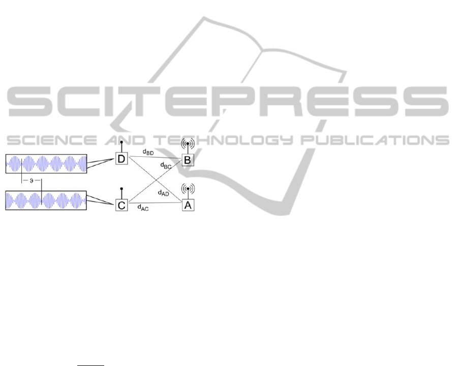
schematics of the radio interferometric measurement
are shown in Figure 1. In the measurement process
two transmitters (A and B) are used, which transmit
only carrier signals (sine waves) with frequencies
and
, respectively. The carrier frequencies are set
to be close to each other, thus a low frequency
interference signal is produced at two receivers,
denoted by C and D in Figure 1. The frequency of
the interference signal is ∆
|
|
at both
receivers, but its phase depends on the relative
positions of the transmitters and the receivers. This
phase difference is used to provide position
estimates.
Figure 1: Radio interferometric measurements.
Note that the interference signal is actually the
received signal strength (RSSI), which can be
measured in most RF transceivers. By providing
time synchronization between receivers C and D, the
phase difference between the RSSI signals of the
receivers can be measured. The phase difference
can be expressed as a function of the relative
positions of the transceivers and receivers, as
follows:
2
/
2
(1)
where is the carrier frequency (
), is
the speed of light, the pairwise distances
,
,
, and
are defined in Figure 1, and
the quantity
is the following linear
combination of the pairwise distances:
.
(2)
Note that in (1) the phase values are wrapped,
(02, thus the exact value of
cannot
be expressed from a single phase measurement. In
(Maroti, 2005) the phase ambiguity problem is
addressed by using multiple carrier frequencies,
providing multiple measurements. Solving
Diophantine equations of values the exact
value of
can be calculated. The proposed
method in (Maroti, 2005) works well if the error of
is small, thus RIPS required long measurements
(80 minutes of data collection time was reported in
(Maroti, 2005)).
In our proposed solution we do not try to resolve
the phase ambiguity problem at one position, rather
we use only the wrapped phase values and resolve
the ambiguity problem with multiple measurements
at different positions, as the object moves. Thus the
proposed solution is suitable for tracking, but not for
localization.
3 PROPOSED SOLUTION
The proposed solution offers two operation modes:
Mode 1: on-line tracking of objects with known
initial position. In this mode the movement of the
object is tracked in real-time from the known initial
position.
Mode 2: off-line tracking of objects with
unknown initial position. In this mode a sufficiently
long data must be recorded, while the object moves;
after sufficient amount of data is collected the full
object track is determined (retroactively) and the
tracking can be continued as in on-line Mode 1.
Since Mode 1 is a subcase of Mode 2, we will
discuss only the operation of Mode 2 in detail.
3.1 Requirements
The proposed solution has some realistic
assumptions and requirements, as follows:
R1: The exact positions of the infrastructure
nodes are known.
R2: The movement of the object is slow,
compared to the sampling frequency. According to
experiments, the object should not move more than a
few tens of millimeters between two consecutive
phase measurement rounds.
R3: The object trajectory is long enough to allow
the resolution of the ambiguity problems (Mode 2
only). There is no explicit known formula yet on
how long the trajectory should be; according to our
experiments the more complex the movement
(containing multiple directions) the shorter trajectory
is enough. See the simulations and the measurement
result is Section 4.
R4: The initial object position must be known
(Mode 1 only). In Mode 2 the initial position is
Radio-InterferometricObjectTrajectoryEstimation
269

unknown and is determined by the algorithm.
3.2 Tracking Infrastructure
The tracking infrastructure contains transceivers at
known positions, which can either play the role of
transmitters to generate interference signals at the
receivers, or receivers to allow phase difference
measurements, as described in Section 2. The
tracked node is always a receiver. Infrastructure
nodes alter their roles, thus different interference
signals can be generated.
A simple measurement uses three infrastructure
nodes (two transmitters and one receiver) and the
tracked receiver node, in a measurement
configuration. The four nodes in the configuration
can measure a phase difference value , which
depends on the positions of both the infrastructure
nodes and the tracked node. Such simple
measurements are carried out with different
configurations, to provide a measurement round,
containing simple measurements. The
measurement results of a complete round will be
used as inputs in each step of the tracking algorithm.
Figure 2 illustrates a scenario with four fixed
nodes A, B, C, D, and one tracked node X. In this
case
12 possible configuration exists, as
shown in the table of Figure 2.
3.3 Position Confidence Map
In each configuration 1,2,…, the ideal
phase values
can be calculated for every
possible object position , using (1) and (2). For two
dimensions, this gives a 2D phase map. Note that
phase maps can be pre-computed and stored, to
increase the speed of the algorithm.
Measurement round produces phase
measurements, each measurement corresponding to
one measurement configuration, as follows:
Figure 2: An example tracking infrastructure with for
fixed nodes (A, B, C, D) and one tracked node (X). The
possible configurations are listed in the table.
,
,…,
(3)
Using the ideal phase maps and the measurements, a
phase offset is calculated for each scenario , as
follows:
∆
,
min
,,
2
(4)
Note that the phase offset values ∆
are between 0
and . From the phase offsets an error map is
calculated, as follows:
,
1
∆
,
(5)
The error is zero if the measurements exactly
correspond to the ideal values; and the maximum
error is 1, indicating large difference between the
ideal and measured phase values. Thus from the
error map a confidence map can be defined, as
follows:
,
1
,
(6)
Confidence value
,
close to one indicates
that position can indeed be the real object position
in time instant , while low confidence values show
that it is unlikely that the object is in position in
time instant .
Figure 3 shows a confidence map computed for a
scenario similar to the one shown in Figure 2. The
true object position is at the center of the figure.
Figure 3(a) shows the case when there is no
measurement noise; in this case there are significant
and sharp peaks in the confidence map. Note that in
this case the confidence value is exactly 1 at the true
object position, but there are several other
significant peaks at phantom positions. This
phenomenon is due to the phase wrapping in (1), and
thus the true object position cannot be determined
from one measurement. The noisy case is shown in
Figure 3 (b), where the peaks are less high and
somewhat blurred. The phantom positions are
clearly observable here as well.
An important observation, which is the basis of
the proposed algorithm, is the following: the true
object location has high confidence value all along
the track of the object (exactly one in noiseless case,
and close to one in noisy case). The phantom
positions, however, change their confidence values,
as the object moves along its trajectory. This
phenomenon is quite salient when a series of
confidence maps is observed: the peak,
corresponding to the true object position, is moving
along the object trajectory; at the same time the
phantom peaks fade and new phantoms appear, only
SENSORNETS2014-InternationalConferenceonSensorNetworks
270
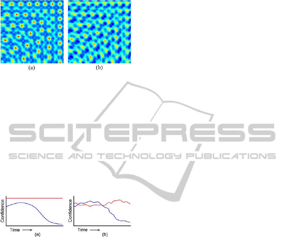
Figure 3: Calculated confidence map for (a) noise free and
(b) noisy measurements. Red colors show high confidence
values, dark blue denotes low confidence values. The true
position is at the center, the other peaks represent phantom
positions.
few phantoms living longer than a few meters.
The phenomenon is illustrated in Figure 4, where
the confidence values, corresponding to the true and
a phantom position, are denoted by red and blue
lines, respectively. Note that in noisy case the
confidence value of a phantom position may be
higher than that of the true position. The phantom’s
confidence, however, will eventually decrease. Thus
the tracking algorithm monitors the (true or
phantom) trajectories, and keeps only those, which
have steadily high confidence values.
Figure 4: Illustration of phase confidence values at the real
(red line) and a phantom (blue line) position of a moving
object, as a function of time. (a) ideal, noise free case, (b)
noisy case.
3.4 Tracking Algorithm
The input of the tracking algorithm in each time
instant (1,2,…,) is the measured phase
vector
, where the vector contains phase
measurements, corresponding to the utilized
configurations, see (3). The output of the algorithm
is the actual track list (atrack), which ideally
contains one and only one track. At the beginning of
the algorithm several possible starting points are
identified: the true one and many phantoms. As the
object moves and new measurements are available,
the algorithm checks whether the current tracks can
be continued, according to the new measurements,
or not. A track can be continued if a possible
location (true or phantom) is close enough to the end
of the track. The required maximum distance is
defined in variable limit. Tracks which cannot be
continued (thus proved to be phantom tracks) are
removed from the actual track list and are stored in
list phtrack. The list of the actual tracks is thus
shrinking, as the moving object provides more and
more information to resolve ambiguities, and finally
contains only the true track alone. The pseudo-code
of the algorithm is the following:
input: ϑ_meas(k), k=1..N
output: atrack, phtrack
Initialization:
atrack = {}
phtrack = {}
map = confidence_map(ϑ_meas(1))
points = possible_positions(map)
for each p points
t= new Track
t.add(p)
atrack = atrack t
Tracking:
for each ph ϑ_meas(2..n)
map = confidence_map(ph)
points = possible_positions(map)
for each t atrack
[d, p] =
min_distance(t.last_point, points)
if d < limit
t.add(p)
else
atrack = atrack \ t
phtrack = phtrack t
The helper functions in the algorithm are the
following:
confidence_map(phase_values)
: calculates
the confidence map for a given phase measurement
set, corresponding to one time instant. See Figure 3.
for illustration of a confidence map.
possible_positions(map)
: analyses the
confidence map and determines possible positions.
In the current implementation we use a hard
threshold confmin to select the high peaks in the
map, then a blob analysis is run to determine the
connected areas, finally the center of each area is
selected as possible position.
min_distance(p, pv)
: from a vector of
points pv selects the closest point to a point p.
Returns both the closest point and the distance.
Radio-InterferometricObjectTrajectoryEstimation
271
4 EVALUATION
In this section the proposed method will be
evaluated using simulations and real measurements.
In the simulations and the real measurements a 4-by-
4 meter area was used where the four infrastructure
nodes were placed into the corners, i.e. the fixed
nodes were placed at positions (0, 0), (0, 4), (4, 0),
and (4, 4), respectively. In all the experiments six
configurations were used, corresponding to
configurations C1…C6 in Figure 2.
First a simulated moving object will be tracked
using various levels of phase measurement error.
Then a proof-of-concept tracking test will be
presented using real measurements.
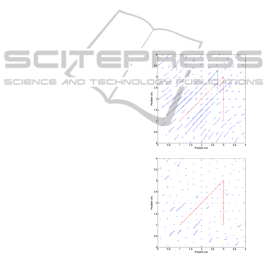
4.1 Tracking Simulations
The proposed algorithm was tested with a simulated
object trajectory, which started from position (1, 1),
moved to (3, 3) and then moved to (3, 1). To the
ideal phase values various amount of additive phase
noise was added to simulate noisy measurements. In
the two experiments zero-mean normal distribution
noise was used with 0.1 and 0.2,
respectively. In both simulations parameters confmin
and limit were set to 0.8 and 0.1m, respectively.
The results of the tests can be seen in Figure 5,
where red lines represent the identified true object
track, while blue lines show the phantom
trajectories. Blue dots show the starting track
positions.
As can be seen in Figure 5, from the initial
tracking positions phantom tracks of various lengths
were detected. Note that the directions of the real
and phantom tracks were approximately the same.
Also note that in the noisier simulation the phantom
tracks are much shorter, because the same confmin
threshold for lower confidence values (see Section
4.1) results an earlier abortion of phantom tracks.
The length of the true trajectory is 400.
With 0.1 the five longest phantom tracks have
285, 228, 116, 108, and 98 points, while with
0.2 their corresponding lengths are 35, 35, 25,
19, and 19 points. The number of starting points
somewhat decreased in the noisier experiment from
164 to 143. This is again due to the fact that fewer
initial points exceeded the same confidence limit.
The accuracy of the position estimation was also
evaluated in the simulations. In the 0.1 case
the maximum, average and the standard deviation of
the estimation error are 25.2mm, 8.3mm, and
18.6mm, respectively. In the 0.2 case the
maximum, average and the standard deviation of the
estimation error increased to 59.9mm, 17.0mm, and
19.1mm, respectively.
4.2 Measurement Results
To test the proposed method a real measurement was
also performed. The used special dual-radio nodes
are based on Atmel’s ATmega128RFA1
microcontroller, equipped with an integrated 2.4GHz
transceiver. The other radio chip is a Silicon Lab’s
Si4432 transceiver, which was used for the radio
interferometric measurements. During the
measurements we used the 868 MHz ISM frequency
band and fine-tuned the radios with the available
312,5 Hz accuracy. The synchronized receivers
performed phase difference measurement on the
RSSI data, sampled with frequency of 62.5 kHz.
(a)
(b)
Figure 5: Simulation result with various measurement
phase noise. The standard deviation of the additive noise
was (a) 0.1 and (b) 0.2. Active and phantom
object trajectories are shown with red and blue lines,
respectively. Blue dots present the initial starting positions
of the tracks.
SENSORNETS2014-InternationalConferenceonSensorNetworks
272
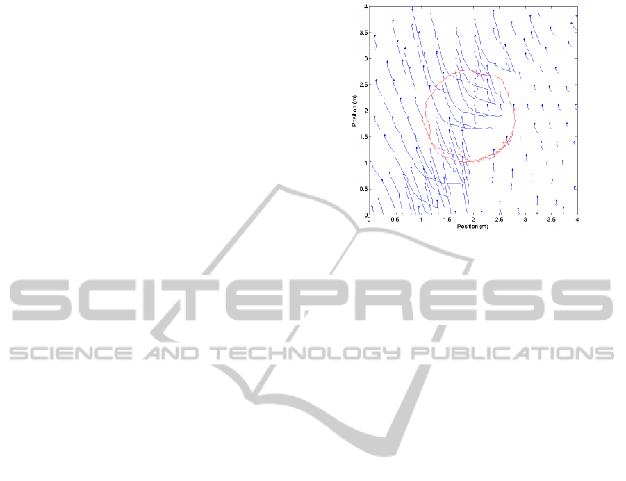
In the test, shown in Figure 6, four nodes and six
configurations were used, as was described at the
beginning of Section 4. Each of the devices were
placed 1.25m above ground level and the tracked
node was carried in hand by a person. The test took
50 seconds while 271 rounds were measured
(altogether 1626 phase measurements were
performed).
The tracking algorithm was executed with
parameter values of limit = 0.1m, and confmin = 0.6.
Initially 169 possible locations were found.
The length of the actual track is 271, as shown in
Figure 6, with red line. The longest five phantom
tracks have lengths of 86, 71, 69, 69, and 69 steps.
4 CONCLUSIONS
In this paper a novel radio-interferometric object
tracking method was proposed. In contrast to former
radio-interferometric localization methods, the
proposed solution resolves the location ambiguity
while the object is moving and provides more and
more measurements.
The proposed solution is able to determine the
full track of a moving object, after the object has
covered a sufficiently large trajectory. Alternatively
it can follow the trajectory of an object in real time,
if the original position of the object is known.
The performance of the algorithm was tested in
simulations and real measurements. The proposed
method, according to simulation experiments, is
robust when the measurement noise is moderate.
The algorithm performed also well in a measurement
using prototype equipment.
Although the preliminary results are very
promising there are several open questions. It is not
known yet how long trajectory the object should
cover before all ambiguities can be resolved. The
dependence of the minimal trajectory length on
various system parameters is also unknown. The
current measurement rate (approximately 5 rounds
per second) should also be improved to allow
tracking of faster objects.
Possible improvements include acceleration of
confidence map generation with GPU based parallel
computing. Currently a simple image processing
algorithm is used to identify the possible locations;
with a tailor-made adaptive algorithm the
performance of the algorithm possibly can be
improved. The robustness of the tracking can also be
increased using model based approaches e.g.
Kalman-filtering.
Figure 6: Output of the tracking algorithm based on a real
measurement. The computed real object track is shown by
red line, while the phantom tracks are shorter blue lines.
The initial track positions are denoted by blue dots.
ACKNOWLEDGEMENTS
This research was supported by the Hungarian
Government and the European Union and co-
financed by the European Social Fund under projects
TÁMOP-4.2.2.A-11/1/KONV-2012-0073 and
TÁMOP-4.2.2.C-11/1/KONV-2012-0004. Gergely
Zachár was supported by the European Union and
co-financed by the European Social Fund in the
framework of TÁMOP 4.2.4. A/2-11-1-2012-0001
'National Excellence Program'.
REFERENCES
Ajdler, T., Kozintsev, I., Lienhart, R., Vetterli, M., 2004.
Acoustic source localization in distributed sensor
networks. In Conference Record of the Thirty-Eighth
Asilomar Conference on Signals, Systems and
Computers, Vol.2, pp.1328-1332.
Au, A. W. S., et al, 2012. Indoor Tracking and Navigation
Using Received Signal Strength and Compressive
Sensing on a Mobile Device. IEEE Transactions on
Mobile Computing, Aug. 2012.
Comaniciu, D., Ramesh, V., Meer, P., 2003. Kernel-based
object tracking. IEEE Trans. Patt. Analy. Mach. Intell.
25, pp. 564–575.
Maroti M., et al, 2005. Radio Interferometric Geolocation.
In ACM Third International Conference on Embedded
Networked Sensor Systems (SenSys 05), San Diego,
CA, pp. 1-12.
Schwarzer, S., Vossiek, M., Pichler, M., Stelzer, A., 2008.
Precise distance measurement with IEEE 802.15.4
(ZigBee) devices. In 2008 IEEE Radio and Wireless
Symposium, pp.779-782.
Radio-InterferometricObjectTrajectoryEstimation
273
