Annotated Trees and their Applications to XML Compression

Tomasz M

uldner

, Jan Krzysztof Miziołek

and Tyler Corbin

Jodrey School of Computer Science, Acadia University, Wolfville, B4P 2A9 NS, Canada

Faculty of Artes Liberales, University of Warsaw, Warsaw, Poland

Keywords:

XML, Tree Compression using Annotated Trees, Permutation-based XML Compression.

Abstract:

Permutation based XML-conscious compressors permute the input document to improve the compression

ratio and support efﬁciency of operations, such as queries or updates. One such compressor, XSAQCT, uses

the properties of the permuted document, called an annotated tree, to these operations. This paper provides

the formal background for the deﬁnition of an of D. It also provides an algorithm for creating an annotated

tree for the XML document and its reverse algorithm, and discusses a measure of compressibility using an

annotated tree. The theoretical and algorithm approaches are followed by the experimental results showing

compressibility of annotated trees and a general analysis of semi-structured data and XML compression.

1 INTRODUCTION

A tree is one of the most important and popular

structures in computing, used to represent the re-

lations between nodes. Therefore, there has been

considerable research on succinct representation of

trees while allowing various operations on these

trees to be efﬁciently performed, see (Chen and

Reif, 1996), (Bille et al., 2013), (Jacobson, 1989)

and (Benoit et al., 1999). The eXtensible Markup

Language, XML (XML, 2013), is one of the most

popular data formats for the serialization of tree

data structures and for the storage of relational data.

Since XML documents are hierarchal and acyclic

in nature, there have been numerous attempts to

apply techniques used for general tree compression

to XML, see e.g., (Busatto et al., 2005), (Ferragina

et al., 2009) and (Busatto et al., 2008). A speciﬁc

subset of tree-compressors designed speciﬁcally for

XML (or semi-structured data in general) are called

XML-conscious compressors, e.g., XQueC (Arion

et al., 2007). These compressors typically parse the

XML, and either sequentially build a model during

compression or build a model and then compress

the contents. XML-conscious permutation-based

compressors permute the input document during a

pre-order traversal and apply a partitioning strategy

to group content nodes into a series of data containers

compressed using a general-purpose compressor (a

back-end compressor). For example, XML compres-

sor XSAQCT is a permuting and streamable XML

compressor, see (M

uldner et al., 2009). The compres-

sion starts with SAX-based parsing to permute the

input into a compressed form of the XML tree, called

an annotated tree. Then it is followed by storing data

values in data containers and compressing data using

a back-end compressors (such as GZIP (GZIP, 2013)

or BZIP2 (bzip2, 2013)).

The annotated tree in XSAQCT can be considered

to be a high level index, which was proved to be

useful for various applications, e.g., updates, online

rather than ofﬂine compression see (Corbin et al.,

2013), and parallelization of the implementation.

However, the formal deﬁnition of this mapping was

never provided nor was the proof that it can be

reversed. These questions are very important because

without answering them, the compression process

used by XSAQCT is not known to be lossless. This

paper ﬁlls in these gaps, by providing a formal

deﬁnition of a tree and an annotated tree, and the

mapping τ from a labelled tree to the annotated tree,

as well as the proof that τ is injective and can be

inverted. An algorithm to create an annotated tree and

its reverse are provided, followed by the discussion

of the compressibility measure of this approach along

with experimental results and a general analysis of

XML compression.

Contributions. There are several novel contribu-

tions of this paper: (1) The theoretical part, i.e., the

formal background for the deﬁnition of an annotated

tree and a proof that the mapping from a tree to the

Müldner T., Miziołek J. and Corbin T..

Annotated Trees and their Applications to XML Compression.

DOI: 10.5220/0004839900270039

In Proceedings of the 10th International Conference on Web Information Systems and Technologies (WEBIST-2014), pages 27-39

ISBN: 978-989-758-023-9

 2014 SCITEPRESS (Science and Technology Publications, Lda.)

annotated tree is injective, and therefore, the anno-

tated tree for the labelled tree D provides a faithful

representation of D; (2) An application of of the an-

notated tree methodology with respect to XML, i.e.,

a formal proof that XSAQCT’s compression process

is lossless; (3) The algorithmic approach, i.e., the al-

gorithm which inputs an arbitrary (cyclic or not) tree

and outputs an annotated tree, and the ”inverse” al-

gorithm for XML, which inputs an annotated tree for

the XML document, and outputs this document; (4)

Quantiﬁcation of text trees and a discussion of mutual

information; (5) A compressibility measure deﬁning

the cost of using annotated trees and results of test-

ing using an especially designed XML suite, show-

ing high compressibility; and (6) General analysis of

XML compression.

This paper is organized as follows. Section 2 in-

troduces the formal background for this paper, includ-

ing a deﬁnition of a tree and an annotated tree. Sec-

tion 3 provides a description of trees with text el-

ements. Section 4 provides algorithms implementing

various mappings and shows time complexity of these

algorithms. Section 5 provides results of testing and a

general analysis, and ﬁnally Section 6 provides con-

clusions and describes future work.

2 TREES AND ANNOTATED

TREES

2.1 Labeled Trees

Deﬁnition 1. Let Σ be an alphabet, called the label

alphabet. A labeled tree is an ordered tree with nodes

labeled by strings from Σ

∗

and having arbitrary de-

grees (i.e., number of children).

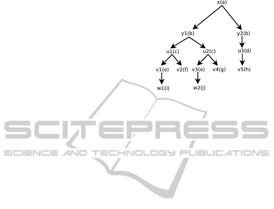
In what follows, by a tree we mean a labeled tree,

and by Trees we denote the set of all trees. We use

the letter D to denote a tree, with nodes denoted by

lower-case letters x, y, u,v (with indices when needed)

and by x(a) we denote a node x labeled with a. Let

Label(x) denote the label of the node x, Height(D)

denote the height of D, Nodes(D) denote the set of

all nodes of D, and D

be the tree consisting of all

nodes and edges in D at levels 1,.. .,i,where1 ≤ i ≤

height(D). Example of a tree is shown in Figure 1.

Deﬁnition 2. A path in a tree is deﬁned to be of the

form /x

,.. . ,/x

, where x

is the root of D and for

1 ≤ i < k,x

i+1

is a child of x

We use a lower-case letter p (with indices when

needed) to denote a path and Paths(D) to denote the

set of all paths in D. For the path p = /x

,.. . ,/x

let Length(p) be the number of nodes in the path p,

Figure 1: Example of a tree D.

Last(p) be the last element x

, Label(p) = Label(x

)

be the label of p, and for Length(p) > 1, let p↓ be the

path p except the last element.

Deﬁnition 3. Two paths in the tree D, p

.../x

and p

= /y

.../y

are called sim-

ilar if k = n, x

= y

is the root of D and for 1 ≤ i ≤

k, Label(x

) = Label(y

The similarity relation is an equivalence relation

and we denote by JpK the equivalence class of p, by

Similar(D) the quotient set of this relation, i.e., the

set of all different sets of similar paths. For p ∈

Paths(D) let Length(JpK) = Length(p) be the length

of the equivalence class, Label(JpK) = Label(p) be

the label of the class (it is easy to see that both def-

initions of the length and the label of an equivalence

class are well deﬁned, i.e., independent of the choice

of the path p from the equivalence class). Finally, for

q ∈ Similar(D) let |q| be the number of paths in q,

and Last(q) be the sequence of nodes that are last el-

ements of all paths in this class, ordered from left to

right. Clearly, |Last(q)| = |q|.

In Figure 1, Similar(D) = {J/xK, J/x/y

J/x/y

K, J/x/y

J/x/y

K, J/x/y

J/x/y

K,J/x/y

K} and for

p = /x/y

,JpK = {/x/y

,/x/y

}; Length(JpK) = 2,

Label(p) = b, Last(JpK) = <y

>, and |JpK| = 2.

Deﬁnition 4. A partial relation ≺ in the set

Similar(D) is deﬁned as follows: Jp

K ≺ Jp

iff Length(Jp

K) = LengthJp

K) > 1, Jp

↓K =

↓K,Label(Jp

K) is different from Label(Jp

K),

and there exist paths p1 ∈ Jp

K and p2 ∈ Jp

K such

that the node Last(p1) is the left sibling of the

node Last(p2). The tree D has a cycle if there exist

∈ Similar(D) such that q

≺ q

and q

≺ q

. D

is acyclic if it does not have a cycle.

For D in Figure 1, J/x/y

K ≺

J/x/y

K, while J/x/y

K and J/x/y

K are

WEBIST2014-InternationalConferenceonWebInformationSystemsandTechnologies

not in relation ≺. There would be a cycle in D if

there was a node u

(e) between nodes u

and u

. By

Acyclic we denote the set of all acyclic trees.

When it does not lead to confusion, a tree can be

represented using a simpliﬁed notation (used e.g. for

XML), by omitting node names, e.g., replacing y

(b)

by b

. In this notation, an equivalence class JpK will

be denoted using the label Label(JpK), in upper case,

e.g., for D from Figure 1, J/x/y

K will be de-

noted by E.

2.2 Annotated Trees and g-trees

A tree D can permuted to create an annotated tree

with nodes represented by equivalence classes of the

similarity relation. In the worst case, if for each

q ∈ Similar(D), |q| = 1 then the size of D would be

the same as the size of the corresponding annotated

tree. However, typically XML documents are regular,

i.e., for majority of paths q ∈ Similar(D), |q| ≫ 1 and

the annotated tree provides a compressed representa-

tion of D. For a single tree D, there may be more than

one annotated tree such that each such annotated tree

can be mapped back to D. To formalize this idea, in

this section we deﬁne annotated trees and annotated

g-trees. Then we deﬁne two mappings, an injective

mapping from the set of trees to the set of annotated

g-trees and an injective mapping from the set of anno-

tated g-trees to set of subsets of annotated trees. Fi-

nally, we deﬁne annotated text trees and a mapping

from text trees to the annotated text trees. In this sec-

tion we consider only acyclic trees, but in Section 4

we provide algorithms for all types of trees. In what

follows, by a dag we mean an acyclic digraph.

Deﬁnition 5. An annotated tree is an ordered tree

with nodes additionally labeled by annotations (se-

quences of non-negative integers). An annotated g-

tree is an unordered tree A (i.e., children are not or-

dered) such that (1) nodes of A are dags; (2) each

dag G ∈ Nodes(A) except the root has its nodes an-

notated; and (3) for every node H ∈ Nodes(A) and

for every child G of H there exists exactly one node

n ∈ Nodes(H), called the source of G, and different

children of H have different sources.

Nodes in the annotated tree are denoted by upper-

case letters (with indices where appropriate), e.g.,

X(n)[α

,.. . ,α

] denotes a node X labeled with the

label n and annotation [α

,... ,α

] or in a simpliﬁed

notation it is denoted as the node N[α

,... ,α

]. Let

AnnotationSum(X) =

∑

i=1

be the sum of all an-

notations of the node X . By Annotated we denote

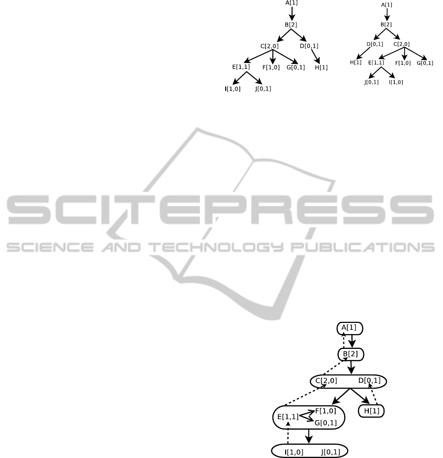
the set of all annotated trees. Two examples of an-

notated trees (using a simpliﬁed notation) are shown

in Figure 2 and Figure 3. As we will explain it later,

Figure 2: Annotated tree.

Figure 3: Another an-

notated tree.

both these trees represent the same tree D from Fig-

ure 1. Example of an annotated g-tree is given in Fig-

ure 4 (the source of a node is shown using a dashed

arrow). By Annotated−G we denote the set of all an-

notated g-trees and by a chain we mean a rooted dag

such that each node except the root has the in-degree

one and each node except one designated node called

the sink has the out-degree one; the sink has the out-

degree zero. The reason for deﬁning g-trees is that

a dag G, which is a chain, will have its nodes repre-

senting children of the source (in left-to-right order)

of G. If a dag G is not a chain then G needs to be

topologically sorted for our usage. For example, in

Figure 4 the topological sorting of the dag containing

nodes E, F and G may produce the chain E,F,G and

these three nodes can be made children of the source

of this graph, i.e., the node C.

Figure 4: Example of a g-tree.

2.3 Tree Isomorphism

Since we will show that the mapping from the set of

trees to the set of g-trees is injective, we need to deﬁne

the concept of ”identical” or isomorphic trees, which

differ only in names of the corresponding nodes. We

use a similar concept for annotated trees and g-trees.

Deﬁnition 6. Two trees D

and D

are isomorphic iff

they have the same height h and for each level i, 1 ≤

i ≤ h, the sequence of all nodes <n

,... ,n

> (in left-

to-right order) in D

at level i and the sequence of all

AnnotatedTreesandtheirApplicationstoXMLCompression

nodes <m

,... ,m

> (in left-to-right order) in D

level i,k = j, and for 1 ≤ r ≤ k, nodes n

and m

have

the same degree and label.

2.4 Mapping Trees to Sets of Annotated

Trees

We deﬁne the mapping τ : Acyclic→ Annotated−G

in two steps; ﬁrst for nodes and the tree structure, and

then for annotations of nodes. Nodes in all dags are

represented by equivalence classes of the similarity

relation and written as JpK(Label(p))[α

,.. . ,α

] or

using a simpliﬁed notation Label(p)[α

,... ,α

]. If x

is a node in D, which is not a root, then by p

denote a (unique) path p ∈ Paths(D) which ends in x.

Deﬁnition 7. Deﬁnition of mapping τ :

Acyclic→Annotated−G. Let D ∈ Acyclic.

• Mapping labeled nodes and the tree structure

1. The root r of D is mapped to the root of τ(D)

deﬁned as a graph consisting of a single node

J/rK(Label(r )).

2. For any level i > 1 of D and equivalence

class q ∈ Similar(D) of length i − 1 let N

q, i

denote the set of nodes x in D at level

i such that Jp

↓K ∈ q. Clearly, the sets

q, i

: q ∈ Similar(D)} form a disjoint cov-

erage of the set of all nodes in D at level i.

Each set N

q, i

is mapped by τ to the single

graph G ∈ Nodes(τ(D)) at the level i; G =

{Jp

K(Label(p

)} where the source of G is the

node q. For any graph G ∈ Nodes(τ(D)) and

two nodes q

∈ G, there is an edge q

=⇒q

in G iff q

≺q

, (see Deﬁnition 4). Since D is as-

sumed to have no cycles, G is acyclic. The node

H ∈ Nodes(τ(D)) is the parent of the node G if

the source of G belongs to the dag Nodes(H).

From the deﬁnition of sets τ(N

q, i

),H is the

unique parent of G.

• Annotations are deﬁned by induction on the height

of τ(D)

1. The annotation of the root is [1]

2. Assume that annotations are deﬁned up to

the level i, 1 ≤ i < Height(D) and for any

equivalence class q of length i, |Last(q)| =

AnnotationSum(q), i.e., the sum of all anno-

tations for the node q is equal to the num-

ber of last elements in all paths in this class.

Consider a dag G at the level i + 1 with the

source X, and a node Y ∈ Nodes(G). Let

Y = JpK(r)[α

,.. . ,α

],X = Jp↓K(m) and k =

AnnotationSum(X). First, we set the number

j of annotations in Y to be k. From the in-

ductive assumption it follows that the sequence

Last(Jp↓K) has k elements s

,.. . ,s

. For 1 ≤

j ≤ k, we deﬁne α

to be the number of chil-

dren in D of the node s

which are labeled

with r. It is easy to see that |Last(JpK)| =

AnnotationSum(Y).

Let Trees

denote the image τ(Acyclic) ⊂

Annotated−G. From the Deﬁnition 7, it follows that

any g-tree A ∈ Trees

, A = τ(D) has the following

properties:

1. Height(D) = Height(A)

2. For 1 ≤ i ≤ Height(D),D and A have identical sets

of labels at level i

3. For a dag G ∈ Nodes(A), let X be the source of

G,X = JqK and k = AnnotationSum(Y ). Then for

each node Y ∈ Nodes(G), Y = JpK(n)[α

,... ,α

]

there exists i,1 ≤ i ≤ k such that α

> 0; j = k, and

Jq↓K = JpK

4. If a node q is not a source of any dag, then all

nodes in the sequence Last(q) are leaves in the

tree D.

For the tree D from Figure 1, the g-tree τ(D) is

shown in Figure 4. From Property 1 it follows that the

height of a g-tree for the document D is the same as

that of D; however typically these trees have different

width and therefore represent a compressed form (see

more in Section 5).

Theorem 1. The mapping τ : Acyclic→Trees

is in-

jective.

Proof. We will deﬁne the mapping τ

−1

Trees

→Acyclic such that τ

−1

◦τ = τ◦τ

−1

is an

identity mapping, i.e., it maps a tree to an isomorphic

tree. Let A ∈ Trees

. Then τ

−1

is deﬁned inductively

on levels i of A:

1. for i = 1, let the root of A be a graph G consisting

of a single node X(a)[1]). Then τ

−1

(G) = x(a)

2. Assume that for all levels i,1 < i <

Height(A), D

= τ

−1

(A)

∈ Acyclic. We de-

ﬁne τ

−1

: A

i+1

→D

i+1

. Let G be a dag in A

at level i + 1, and Nodes(G) = {Y

,··· ,Y

where for j,1 ≤ j ≤ m, Y

= Jq

K(r

)[α

,...,α

the node X = JpK(m) be the source of of G ,

k = AnnotationSum(X), and Last(JpK) be the

tuple s

,...,s

For h,1 ≤ h ≤ k we now deﬁne τ

−1

(G) as nodes

in D at the level i + 1 that are children of each

node s

. First, for j, 1 ≤ j ≤ m , let N

h, j

be the

set of nodes in D at the level i + 1 consisting of

nodes in D labeled by r

. We deﬁne a partial

order between these sets as follows: for j

and

,1 ≤ j

, j

≤ m, N

h, j

≺ N

h, j

iff in G there is

WEBIST2014-InternationalConferenceonWebInformationSystemsandTechnologies

an arc between Jq

K and Jq

K. Finally, children

of s

are nodes from sets N

h, 1

,... ,N

h, m

deﬁned

as follows: (1) within each set N

h, j

, nodes are ar-

bitrarily ordered and appear one after another; (2)

for any two sets N

h, j

and N

h, j

all nodes from

h, j

appear to the left of all nodes in N

h, j

iff

h, j

≺ N

h, j

; and (3) for any set N

h, j

which is

not in the relation ≺, we arbitrarily place children

from this set to appear after all nodes from sets

which are in this relation with another set.

Clearly the tree τ

−1

(A) is acyclic and for D ∈

Acyclic,τ

−1

◦τ(D) = D, for A ∈ Trees

, τ

−1

◦τ(A) =

Next, we deﬁne the mapping γ :

Trees

→2

Annotated−G

. Let T S(G) be the set of

all topological sortings of a dag G, and for G

,··· ,G

P(G

,.. . ,G

) be a Cartesian product ×

i=1

T S(G

If <g

,... ,g

> ∈ P(G

,... ,G

) then each graph g

represents a topologically sorted graph G

Deﬁnition 8. Mapping γ is deﬁned as follows: For

T ∈ Trees

, γ(T ) = {γ

,...,g

(T ) : <g

,.. . ,g

> ∈

P(G

,.. . ,G

)} where γ

,...,g

(T ) is the g-tree T

with all graphs G

,... ,G

replaced respectively by

graphs g

,... ,g

, and having the same arcs between

dags (as well as sources) as in the tree T.

Let Trees

denote the image γ(Trees

) ⊂

Annotated−G

Theorem 2. The mapping γ : Trees

→Trees

is in-

jective.

Proof. We will deﬁne the mapping γ

−1

Trees

→Trees

s.t. γ

−1

◦γ and γ◦γ

−1

are iden-

tity mappings. It is sufﬁcient to show that each

topologically sorted dag g

with annotated nodes can

be uniquely mapped to the dag G

. Two different

nodes X[α

,...,α

] and Y [β

,.. .,β

] from the dag g

will be called dependant if there exists m,1 ≤ m ≤ k

such that α

> 0 and β

> 0. Now, let us deﬁne

−1

) to be the graph consisting of the same nodes

as in the graph g

and with the same source, but with

arcs deﬁned as follows: there is an arc X =⇒ Y iff

the node X appears in the topological sort used in g

before the node Y , and X and Y are dependant.

It is easy to see that each g-tree T ∈ Trees

in one-to-one correspondence with an annotated tree.

Since τ : Acyclic↔Trees

and γ : Trees

↔Trees

each tree D can be mapped to the set of annotated

trees, denoted by Annotated(D) and deﬁned by the

composition of τ and γ. It is easy to see that every

annotated tree from the set Annotated(D) represents

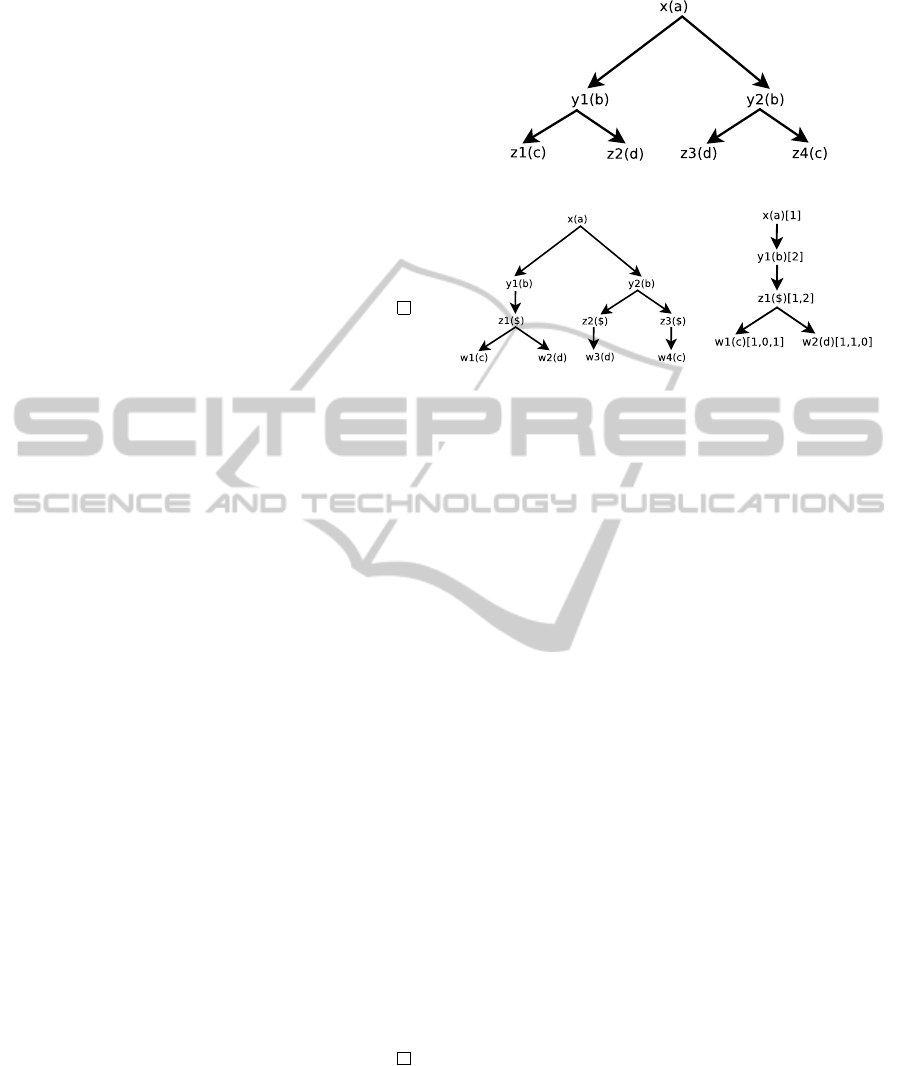
Figure 5: Cyclic Tree.

Figure 6: Acyclic tree with

dummy nodes.

Figure 7: The anno-

tated tree with dummy

nodes.

D. For example, both annotated trees shown in Fig-

ure 2 and Figure 3 belong to the set Annotated(D)

that uniquely represents the tree D.

If there is a cycle in D, then we map D to an

acyclic tree with the so-called dummy nodes, denoted

by $. After adding a dummy node to a cyclic doc-

ument D in Figure 5, this tree will be acyclic, see

Figure 6, and it can be mapped to the annotated tree

shown in Figure 7. We do not formally prove that the

mapping from the tree with cycles to a tree with the

dummy nodes is injective but provide Algorithm 1 in

Section 4 showing how cycles can be removed.

3 TEXT TREES AND THEIR

COMPRESSION

Since the procedure of compressing text trees is al-

most identical to the procedure of compressing la-

beled trees, in this section we provide only the de-

scription of how text nodes are dealt with.

3.1 Text Trees

Deﬁnition 9. Let ∆ be an alphabet, called the text

alphabet, its elements are \0 terminated strings. A

text tree is a tree with two kinds of nodes; element

nodes labeled by strings from Σ

∗

(see Deﬁnition 1)

and text nodes labeled by strings from ∆

∗

such that

text nodes are always leaves, the root of the text tree

is an element node, and any two sibling text-nodes are

separated by at least one element node.

For text trees we use the same notations as for

trees; text labels are denoted using letter t (with in-

AnnotatedTreesandtheirApplicationstoXMLCompression

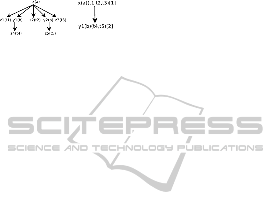
Figure 8: Text tree.

Figure 9: The anno-

tated text tree.

dices if needed), see Figure 8. By TextTrees we de-

note the set of all text trees, and by AcyclicTextTrees

we denote the set of all acyclic text trees. A text tree

can be used to represent an XML document with text

values represented by labels of text nodes. Text nodes

may or may not be present and now we deﬁne com-

plete text trees corresponding to the full-mixed con-

tent of XML documents, see (M

uldner et al., 2012).

Deﬁnition 10. An element leaf node in the text tree is

the element node that has no element child. A text tree

is called complete if every non-leaf element node has

the left and the right text sibling, and every element

leaf node has exactly one text child node.

The text tree from Figure 8 is complete; it would

not be complete if any of the text nodes were miss-

ing. Note that in XSAQCT when the input XML doc-

ument D is parsed then for any missing text node, a

text node labeled by an empty text (consisting of \0

only) is added. To support a unique representation of

an XML document using this technique, added text

nodes are removed while D is restored. In what fol-

lows, we assume that text trees are complete.

3.2 Compressed Representation of Text

Trees

Deﬁnition 11. For a node X in the annotated tree

with m children Y

,... ,Y

, m ≥ 0 let Number(X)

= (

∑

j=1

AnnotationSum(Y

))+AnnotationSum(X). An

annotated text tree is an annotated tree with nodes

additionally labeled by concatenations of strings from

∆

∗

, called text labels, such that a text label T of a node

X(a)(T ) is equal to the concatenation of Number(X )

text labels.

Example of an annotated text tree is shown in Fig-

ure 9. By AcyclicAnnTextTrees we denote the set of

all acyclic annotated text trees.

3.3 Mapping Text Elements

For every equivalence class JpK, labels of text nodes

that are children of element nodes (in left to right

order) from the sequence Last(JpK) will be concate-

nated into a single text label of the node in the anno-

tated tree that corresponds to this equivalence class.

For example, the text tree shown in Figure 8 will

be mapped to the annotated text tree from Figure 9,

where t

denotes a concatenation of texts. The rea-

son for mapping text nodes this way is that for query-

ing of the XML documents, the query of the form /X

returns the concatenated texts appearing in this path.

Deﬁnition 12. Let D ∈ AcyclicTextTrees and let A

be the image of D under τ (see Deﬁnition 7) as if

there was no text nodes in D. Now, for every node

X ∈ A, we will deﬁne its text label T such that the

number of texts concatenated in T will be equal to

Number(X). Let τ

−1

(X), as deﬁned the proof of The-

orem 1, be the sequence x

,.. . ,x

of element nodes,

where k = AnnotationSum(X) and let us consider two

cases:

1. X is a leaf. Then for every 1 ≤ i ≤ k, x

has exactly

one text child, and let T be the concatenation of

labels of these k children. Clearly, Number(X) =

AnnotationSum(X) = k.

2. X is a not leaf, and it has m children, Y

,... ,Y

Thus, there are Number(X) text children of nodes

,... ,x

, and we deﬁne T to be the concatenation

of labels of these children (in left-to-right order).

Theorem 3. The mapping of text elements is injective.

Proof. Let A be an annotated text tree and D be the

text tree; we will describe how text labels from A are

mapped into the text elements in D. Consider the node

X ∈ Nodes(A) and let k = Number(X). The image

of X under the reverse mapping is the sequence of

element nodes x

,...,x

. We consider two cases:

1. X(T ) is a leaf. Then k = Number(X ) =

AnnotationSum(X) and T is a concatenation of k

texts t

,... ,t

. For every i,1 ≤ i ≤ k, we deﬁne a

text child y

) of the node x

2. X(T ) is a not leaf and it has m chil-

dren Y

),... ,Y

), where T is a con-

catenation of r = (

∑

j=1

AnnotationSum(Y

)) +

AnnotationSum(X) texts s

,.. . ,s

. Given a node

x in a tree from AcyclicTextTrees with k element

children y

,... ,y

and k + 1 texts t

,... ,t

, text

nodes are deﬁned as follows: (1) the node labeled

is the leftmost child of the node x, and (2) for

i,1 ≤ i ≤ k, the node labeled t

is the right sibling

of the node y

. Assume that each element node

has n

element children, so r = (

∑

j=1

) + k.

Now, let us create text children of nodes x

,... ,x

using the above method and consecutive groups of

texts from T , i.e., for x

and its element children

,... ,y

we use the ﬁrst n

+ 1 texts from T ,

WEBIST2014-InternationalConferenceonWebInformationSystemsandTechnologies

for x

and its element children y

,.. . ,y

we use

the next n

+ 1 texts from T , etc.

Clearly the tree τ

−1

(A) is acyclic and for D ∈

Acyclic(D),τ

−1

◦τ(D) = D.

4 ALGORITHMIC APPROACH

This section provides the algorithm to create an anno-

tated tree for a ﬁxed labeled tree D, which may or may

not be cyclic. There are two steps in the process of

creating an annotated tree, respectively implemented

by Algorithm 1 and Algorithm 2. After the ﬁrst step,

when parsing of D is performed, for each set of sim-

ilar paths there will be an associated graph of anno-

tated nodes, which may include (in case of a cyclic

input document) a special annotated dummy symbol

. The second step uses data created by the ﬁrst step

to create an annotated tree. We also show the Algo-

rithm 3 for the inverse mapping for XML, which in-

puts an annotated tree for the XML document D and

outputs D.

4.1 Notations and Auxiliary Abstract

Data Types

Recall that x(n) denotes a node x labeled by n in D,

and X(n)[A] denotes an annotated node X labeled by

n with the annotation A. For the path p ∈ P and a

node x ∈ D, let p/x denotes the path p extended by /x,

and X0(p) denotes the so-called current node (which

could be empty). Recall from Section 2.1 that p↓

denotes the path p except its last element, and from

Section 2.2 that AnnotationSum(X) denotes the sum

of all annotations of the node X . Let A(n) denote

a list of AnnotationSum(X0(p↓)) − 1 occurrences of

integer n, i.e., k − 1 occurrences of n, where k is the

sum of all annotations of the current node for the path

p↓. For example, if AnnotationSum(X 0(p↓)) − 1 is

equal to four, then [A(5),1] denotes the annotation

[5,5,5,5,1]. If X is a node or the dummy node then

Inc

(

)

we denote the following modiﬁcation of

the annotation of X: if i = 1 then the last annotation

of X is incremented by one; if i = 0 then ”,0” is added

after the last annotation of the dummy symbol. Let P

be the set of equivalence classes of the similarity rela-

tion (see Deﬁnition 3) maintained by the Algorithm 1

(initially, it consists of the equivalence class for the

path /root of D). For every equivalence class q ∈ P , let

G(q) be a pair consisting of (a graph with annotated

nodes, a dummy node $), and let $(p) denotes the an-

notation of the dummy node for the class JpK. Now,

we deﬁne several auxiliary notations and operations:

(1)

int insertP(path p)

returns 0 if JpK ∈ P ; oth-

erwise it inserts JpK into P , sets G(JpK) to be an

empty graph and empty dummy symbol, and returns

1; (2)

Annotatednode insertG(path p, label

n, annotation A)

; (3)

node memberG(path p,

label n)

returns the unique node X in G(JpK) such

that X is labeled with n; (4)

addArc(node X1, node

X2, path p)

adds a new arc connecting X 1 and X2

in G(JpK); (5)

annotation Ann(path p)

if the path

p is of the form \root or S(X0(p↓)) is equal to 1 then

return 1, otherwise return the annotation S(X0(p↓))-

1 of 0’s, 1; (6)

int reachableG(node X1, node

X2, path p)

returns 1 if the node X2 is reachable

from the node X2 in G(JpK), otherwise it returns 0;

(7)

sortG(path p)

performs a topological sort of

G(JpK); (8)

update(path p)

for each node X in

G(JpK) performs Inc(X,0).

4.2 Mapping a Labeled Tree D to an

Annotated Tree

This section presents Algorithms 1 and 2 which map a

labeled tree D, possibly cyclic, into an annotated tree,

which in case of cycles adds dummy nodes labeled

by $ (thus algorithms in this section are designed for

arbitrary trees, rather than for XML trees). Algo-

rithm 1 performs a depth-ﬁrst search traversal of the

input tree, moving down and up. For the XML docu-

ment D, these actions would be triggered by entering

the beginning of the element, i.e.,

and the end of

the element, i.e.,

</x

. The algorithm maintains the

current path p0 in D, and for each path p in D it main-

tains the set P of paths and associated graphs G(JpK).

It also maintains the current annotated node X0(p) in

G(JpK) and the annotated dummy node.

The Algorithm 1 is initialized by setting the node

x0 to be the root of D and p0 to be the path /x0.

Then it performs a loop moving down and up until it

reaches the root node and there are no more un-visited

children of the root, while maintaing the following

two invariants: (1) The current node X0(p0↓) is not

null; (2) If the algorithm moves down to the node x,

such that the path p/x already exists, then there ex-

ists a unique annotated node X in the graph G(Jp0K)

which has the same label as the label of x. Once the

algorithms complete their actions, the set P stores all

equivalence classes of the similarity relation for D.

Table 1 shows the trace of the execution of Algo-

rithm 1 for the document D from Figure 5, using sim-

pliﬁed notation. The current annotated node X0(p) (if

any) is underlined. If the tuple (path q, G(q)) has not

changed, then it is not shown again. The action of go-

ing down to the node x is shown as ↓x and the action

of going up to the node x is shown as ↑x. Each q ∈ P

AnnotatedTreesandtheirApplicationstoXMLCompression

will represent a node of the annotated tree, and the

annotated nodes from the graph G(q) will represent

children of these nodes. Algorithm 2 inputs the out-

put of the Algorithms 1 and produces the annotated

tree.

Algorithm 1: Algorithm which maps a tree to a set P

and associated graphs.

Require: x0 = root of D, p0 = /x0, G(Jp0K)=(graph and

dummy node; both empty)

1: function TRAVERSE

2: while true do

3: if current is root and no more nodes then

4: return;

5: end if

6: if moving down to x then

7: p1 = p0/x;

8: if insertP(p1) then // p1 is a new path

9: X1 = insertG(p0, label of x, [A(0),1]);

10: if X0(p0) ̸=

0 then

11: addArc(X0(p0), X1, p0);

12: end if

13: else// p1 is already deﬁned

14: X1 = memberG(p0,label of x);

15: if X0(p0) ̸=

0 AND X1 ̸= X0(p0) then

16: // check if arc can be added

17: if !reachableG(X0(p), X1, p0) then

18: // can add

19: Inc(X1,1);

20: update(p1);

21: addArc(X0(p0), X1, p0);

22: if $(p0) ̸=

0 then

23: Inc($ ,0);

24: end if

25: else// needs a dummy node

26: if $(p0) ̸=

0 then

27: Inc($,1);

28: else

29: $(p0) = $[A(1), 2];

30: end if

31: update(p0);

32: Inc(X1,1);

33: end if

34: else

35: X0(p0) = X1;

36: Inc(X1,1);

37: update(p1);

38: if $(p1) ̸=

0 then

39: Inc($ ,0); Inc($ ,1);

40: end if

41: end if

42: end if

43: X0(p0) = X1;

44: p0 = p1;

45: else// moving up to the node x

46: X0(p0) =

47: p0 = p0↓;

48: end if

49: end while

50: end function

Let n be the number of nodes in the input tree.

The Algorithm 1 is based on DFS-traversal of a tree,

which has O(n) time complexity, with the nested call

Table 1: Trace of the execution of Algorithm 1.

Move p0 p1 JpK : G(JpK), dummy

/a A:

↓b1 /a/b1 /a/b1 A: B[1],

↓c1 /a/b1/c1 /a/b1/c1 B: C[1],

↑b1 /a/b /a/b1/c1

↓d1 /a/b1/d1 /a/b1/d1 B: C[1]→D[1],

↑b1 /a/b1/

↑a /a B:, C[1]→D[1],

↓b2 /a/b2 /a/b2 A:Y(b)[2],

B: C[1,0]→D[1,0],

↓d2 /a/b2/d2 /a/b2/d2 B: C[1,0]→D[1,1],

↑b2 /a/b2

↓c2 /a/b2/c2 /a/b2/c2 B: C[1,0]→D[1,1]

B: C[1,0,1]→D[1,1,0]

$[1,2]

↑b2 /a/b2

↑a /a

Algorithm 2: Algorithm which maps a set P and as-

sociated graphs to an annotated tree.

Require: Initially p = \root, X = root(label of the

root of D)[1]

1: function FIN ALIZE(Path p, Node X)

2: if $(p) ̸=

0 then

3: make the node $(p) a child of X;

4: X = $(p);

5: end if

6: Node R = sort(p); // now G(p) is a chain

7: make annotated nodes in G(p) children of X

8: for every node X1 in G(p) do

9: if G(p) ̸=

0 then

10: Finalize(p/(label of X1), X1);

11: end if

12: end for

13: end function

(line 17) to the function reachableG(), which has

O(|V | + |E|) time complexity, where |V | is the num-

ber of vertices in the graph passed as a parameter to

the function, and |E| is the number of vertices in this

graph. Therefore, time complexity of this algorithm is

O(n

). Similarly, Algorithm 2 has O(n

) complexity.

4.3 Mapping an Annotated Tree to the

Labeled Tree

Now we present the algorithm 3, which describes for

an XML document a mapping reverse to the previ-

ously described mapping, i.e., it inputs an annotated

tree (possibly with dummy nodes) and outputs the

XML document. The following notations are used:

(1) ann(n): ﬁrst digit in the annotation of the node n;

(2) chop(n): remove the ﬁrst digit in the annotation of

n (always 0); (3) dec(n): decrement by one the ﬁrst

WEBIST2014-InternationalConferenceonWebInformationSystemsandTechnologies

Algorithm 3: Algorithm which inputs an annotated

tree and outputs the XML document.

Require: Called for the root of the annotated tree

1: function RESTORE(Node c)

2: n = LC(c);

3: while n ̸=

0 do

4: if ann(n) > 0 then

5: if n is not a dummy node then

6: output < + label of n + >;

7: end if

8: Restore(n);

9: else

10: chop(n);

11: end if

12: n = RS(n);

13: end while

14: dec(c);

15: if c is not a dummy node then

16: output </ + label of c + >;

17: end if

18: if ann(c) = 0 then

19: chop(c);

20: else

21: output < + label of n + >;

22: Restore(c);

23: end if

24: end function

digit in the annotation of n (never 0); and (4) LC(n)

and RS(n): respectively the leftmost child and right

sibling of n. Given the annotated tree T, to restore

the XML document, the following actions should be

executed:

output <root label>; Restore(root

of T); output </root label>

Algorithm 3 has

O(n

) complexity.

5 EXPERIMENTAL RESULTS

AND GENERAL ANALYSIS

This section describes an analysis of distribution of

text elements in semi-structured data, and the deﬁni-

tion of a compressibility measure for annotated fol-

lowed by experimental results using an XML suite.

Finally, it provides a general analysis of XML com-

pression.

5.1 Quantiﬁcation of Text Trees and

Mutual Information

The use of annotated representation of a tree T im-

plies the following hypothesis about the distribution

of text elements in the tree: Each equivalence class

in a tree T also deﬁnes a unique random variable

in which the text children are sampled from. The

hypothesis does not imply anything about the mutual

information within the set of random variables;

however, there are some implicit consequences as to

how mutual information is dealt with. Speciﬁcally,

mutual information is the amount of information that

one random variable contains about another random

variable; or the amount of reduction in uncertainty

of one random variable due to the knowledge of

the other. We deﬁne mutual information as I(X|Y),

the reduction in the uncertainty of X due to the

knowledge of Y and consider two general cases in the

transfer of information: (1) [I(Child|Parent

)] - the

transfer of information from a parent node to each

of its children, or the transfer of information from

a N

ancestor to each of its N

descendants; (2)

[

(

Sibling

)

|∀

]

- the transfer of informa-

tion from a sibling node to each of its prior siblings.

Although we cannot explicitly prove any general

relationships of the two clauses above, we can extract

information about the general use of semi-structured

data and their affects on these relationships.

I(Child|Parent): With respect to most semi-

structured data formats, e.g., XML and JSON, the

text of non-leaf elements is mostly the whitespace

data to make the semi-structured data human-

readable, i.e., there is almost no relation between the

information in any parent and the information of a

leaf node. However, there is a clear relation between

the information in any parent and the information

of any non-leaf child. The data is only whitespace,

and we can restrict the text alphabet to ASCII: SPC

(0x20), TAB (0x09), LF (0x0a), VT (0x0b), FF

(0x0c), and CR(0x0d). One caveat to this general

statement, for example, are formatting tags in HTML,

such as

"display <b>bold</b> text"

. However,

in the optimal case, and for semantic equivalence of

the XML, we can functionally, and not statistically,

relate the whitespace characters and the depth of the

node, i.e., the depth multiplied by an indent (tab,

sequence of whitespace, etc.)

I(Sibling

|Sibling

): The relationship among siblings

is slightly more complicated. If we consider the set of

text elements for each equivalence class of leaf nodes,

we can describe similarity between two sets using

Statistical and Alphabetical Similarities, Functional

Relations, and Temporal/Semantic and Structural

Relations. Although statistical and alphabetical

similarities form the basis of our hypothesis about

the relationship of data among individual equivalence

classes, they can also be used describe the relation-

ship of data across equivalence classes. For example,

two nodes:

LastName

and

FirstName

would be

highly informationally related. However, if two tags

consist of only free-formed English, the alphabets

AnnotatedTreesandtheirApplicationstoXMLCompression

may be similar, but the words, sentences, etc. may

be different. Therefore, while there may be some

statistical relationship among the character frequency,

it quickly declines as we increase the degree of our

statistics. Functional relations would describe the

tags whose information is just some deterministic

function of another tag. For example, a

text

tag

and a

sha-256

tag are functionally related. Tempo-

ral/Semantic and Structural Relations, while being

a form of statistical similarity, describe the tags that

have some temporal or sequential relation with its

siblings. Consider this example:

<Q>How many bits to an octet?</Q>

<A>There are 8-bits to an octet.</A>

<A>Generally speaking, 8.</A>

</Questions>

. Although functional relations

can be exploited, they require the relationship to

be known before compression, i.e., there is an

underlying schema to the semi-structured data. Thus,

these type of similarities are often not considered

for general-purpose compression. With respect to

non-leaf children, we expect the data to be quite

statistically (and structurally) similar, because the

data of a sibling set would be consistently formatted

for human readability (or lack thereof). However,

with leaf children, the annotative representation of a

text tree will only exploit the sequence of character

data local to an equivalence class and will not

consider the sequence of character data local to some

subtree (as shown above). Therefore, no compression

algorithm will be able to use the knowledge of “How

many bits to an octet” to compress the information

of ”There are 8-bits to an octet.”. However, to

compress “How many bits to a byte”, we can use the

knowledge of previously asking “How many bits to

an octet”. Therefore, semantically related text of the

same vertex would have a high statistical similarity,

whereas semantically related text of the same subtree

will not be considered for compression.

5.2 Experimental Results

Throughout this section we use the following nota-

tions: D is a tree and A belongs to the set of annotated

trees Annotated(D). Recall from Section 2.2 that this

set uniquely represents D, therefore the description

provided in this section does not depend on the choice

of A. For any tree T (annotated or not), by |T| we de-

note the number of nodes in T . Let the width of D at

any level i be denoted by width(D, i) and let Ann(X)

denote the annotation list of the node X ∈ Nodes(A)

and let |Ann(X)| denote the length of the annotated

list. Finally let X

,.. . ,X

be all nodes in A at level

i (i.e., width(A,i) = N

From the construction of an annotated tree, it fol-

lows that (see also Properties 2.4): (1) width(D,i) =

∑

k=1

AnnotationSum(X

); and (2) In A, for any node

X and its child Y, AnnotationSum(X) = |Ann(Y )|.

Therefore, the larger the sum of all annotations of

X, the longer the annotation list of Y . The implica-

tion of zeros appearing in the annotations of node X

is two-fold: (a) in A, they shorten the length of the

annotation list; (b) in D, Y does not appear as a child

of X. If D was “completely regular” and there were

no missing children, then there would be no 0s on

the annotation lists. From our experiments, it follows

that a leaf annotation lists are usually very long, while

for the leaf’s ascendants, annotations they are getting

progressively shorter. To analyze this phenomenon

consider a leaf node X in A, its parent Y, and Y ’s par-

ent Z (grandparent of X). Since AnnotationSum(Y ) =

|Ann(X)|, the annotation list Ann(X) must have been

increased because of the structure of D, speciﬁcally

Y has “very often” appeared as a child of Z, likely

multiple times (resulting in annotations greater than

1). On the other hand, many 0s appearing in Ann(X )

indicates that X has “very rarely” appeared as a child

of Y .

Let us now consider the compressibility

measure, which measures the cost of storing the

annotated tree A compared to the cost of storing

the original document D. Our deﬁnition is to be

implementation-independent and data are not com-

pressed using a backend compressor. As discussed

before, in general A has fewer nodes than D, but

there is an additional cost of storing annotation lists.

Let C be the cost of storing a single information,

such as a single integer annotation or a node label.

Therefore, the storage cost of a single tree node is

3 × C, and the cost of storing an annotation list of

length L is L ×C. The total storage cost of D is equal

to the cost of storing all nodes in A, including all

annotation lists over the cost of storing all nodes in D,

resulting in

(3×C×|A|)+(

∑

X∈A

|Ann(X)|)×C

3×C×|D|

. Performing

a few simpliﬁcations, gives the following formula

(independent of the cost C):

Deﬁnition 13. The compressibility measure is deﬁned

as follows:

(D) =

|A|+(

∑

X∈A

|Ann(X)|)/3

|D|

In this section we provide experimental results

showing values of the measure from Deﬁnition 13

applied to a suite of XML ﬁles . Characteristics of

these ﬁles are shown in the ﬁrst four columns of Ta-

ble 2, where V(N) denotes the value V*10

, Size

is the size of ﬁle in Bytes, E:A denotes the number

of elements and attributes, AC denotes the number

WEBIST2014-InternationalConferenceonWebInformationSystemsandTechnologies

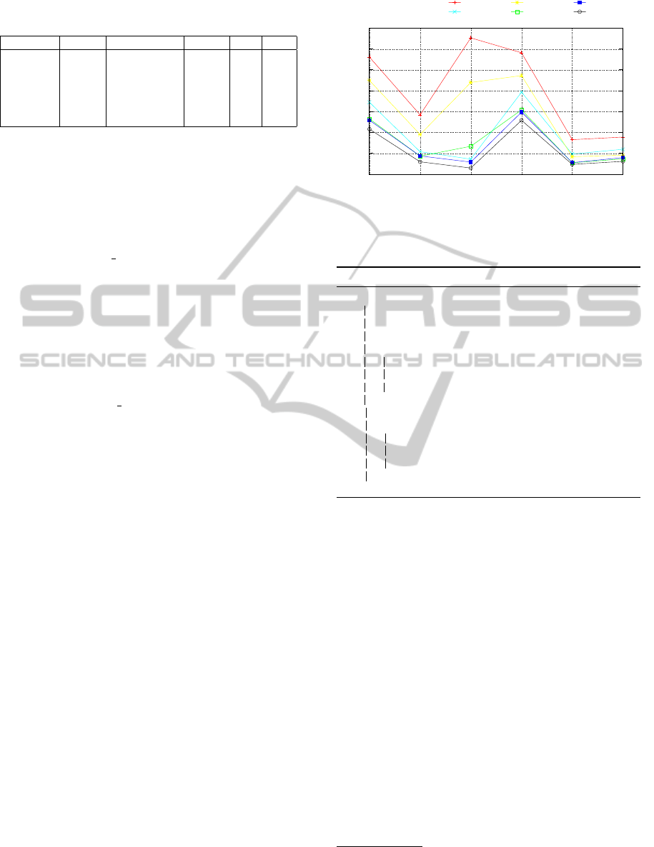
Table 2: Overview of XML Test Suite and Results of Test-

ing.

XML File Size E:A AC AT C

1gig 1.17(9) 1.6(7):3.83(6) 2.05(8) 680 0.41

BaseBall 6.72(5) 2.8(5):0 6.6(5) 47 0.78

enw.books 1.56(8) 5.3(6):4.9(5) 6.38(5) 29 0.40

enw.latest 5.96(9) 1.84(9):1.85(8) 2.59(9) 39 0.47

lineitem 3.22(7) 1.02(6):1 9.6(6) 19 0.31

UniProt 1.15(8) 9.86(5):1.44(9) 1.05(9) 217 0.36

of annotations, AT denotes the number of nodes in

the annotation tree, and C denotes the compressibility

measure. The ﬁles are 1gig.xml (a randomly gener-

ated XML ﬁle, using xmlgen (xmlgen, 2013)), base-

ball.xml (Baseball.xml, 2013), enwikibooks.xml and

lineitem.xml from the Wratislavia corpus (Corpus,

2013), and uniprot sprot (Consortium, 2013). This

suite has been chosen because XML ﬁles included

there have an ability to represent speciﬁc extremes of

semi-structured data. For example, enwiki-latest.xml,

the current revision of English Wikipedia, while being

a very large document, encompasses two extremes:

the distribution of character data is very non-uniform

(i.e., the majority of the data falls within one node)

and that path is predominantly free-formed English.

Conversely, uniprot sprot.xml is a highly uniform

XML ﬁle (i.e., the data is evenly distributed), and the

ﬁle is predominantly markup. The ﬁle 1gig.xml has

the property that the subtree entropy is extremely low

(subtrees are quite similar); however, each subtree dif-

fers by a parent node (for example,

/a/b/d/e/f

vs.

/a/z/d/e/f

). The ﬁle lineitem.xml, has the prop-

erty that it is an incredibly regular tree (few missing

nodes), and in addition, has a nice mixture of text and

numeric data. The ﬁle enwikibooks.xml is quite struc-

turally similar to enwiki-latest.xml but is a fraction of

its size. Finally, baseball.xml is an extremely irregu-

lar XML ﬁle. The last column of the Table 2 shows

the test results, speciﬁcally values of the compress-

ibility measures (see Deﬁnition 13) for the six XML

ﬁle. These results show that the annotated tree pro-

vides a well-compressed representation of the original

ﬁles, even in the presence of very large ﬁles.

5.2.1 Analysis of XML Compression

In measuring the compressibility of the annotated

transform, each XML ﬁle was transferred into three

separate ﬁles: (1) the annotated tree (a list of strings

encoded in depth-ﬁrst ordering); (2) the annotations

(written in depth-ﬁrst ordering); and (3) the text con-

tainers (written in depth-ﬁrst ordering), see Algo-

rithm 4. Consequently, this transform does nothing

but to act as a pre-processor for other text compres-

sors.

Ignoring Kolmogorov complexity (and Kol-

0.05

0.1

0.15

0.2

0.25

0.3

0.35

enlatest

Uniprot

1gig

enwikibooks

Lineitem

Baseball

GZIP

BZIP

PPMonster

ZPAQ

paq8pxd_v7

Figure 10: Compression of entire XML document with sin-

gle instances of Vanilla Compressors.

Algorithm 4: Annotated Process.

1: function ENCODE(AnnotatedTree A, File ﬁle)

2: write(encode(A.schema), ﬁle.schema)

3: DepthFirstIterator dfs

4: // For each node, its annotation list.

5: for (dfs = A.iterator(); dfs.hasNext();) do

6: AnnotatedNode node = dfs.next()

7: write(node.annotationList.length(), ﬁle.annot).

8: write(node.annotationList, ﬁle.annot).

9: end for

10: // For each node write its text container.

11: for (dfs = A.iterator(); dfs.hasNext();) do

12: AnnotatedNode node = dfs.next()

13: write(node.textContainer.length(), ﬁle.text).

14: write(node.textContainer, ﬁle.text).

15: end for

16: end function

mogorov compressors), we assume the XML data

to be distributed according to some random vari-

able (or set of random variables). Therefore, the

ideal way to analyze the compression beneﬁts in-

duced by the annotated transform would be to an-

alyze how much beneﬁt, with respect to the abso-

lute lower bound, was obtained. However, since it

is nearly impossible to calculate the exact entropy of

the XML sources, the next ideal step would be to ap-

proximate the entropy using a lossless compression

algorithm, which would be infeasible for the analy-

sis of the proposed transform. Analyzing the percent-

age increase in compression does not take into con-

sideration how substantial a percent decrease in size

is, but it will be used as the base metric of compari-

son. For this analysis, a series of different compres-

sors were used, see Figure10. LZ77-based (Ziv and

Lempel, 2006) compressors, GZIP

and XZ

, BWT-

based (Burrows and Wheeler, 1994), BZIP2

, Predic-

gzip -9 FILE

xz -9 -e FILE

bzip2 -9 FILE

AnnotatedTreesandtheirApplicationstoXMLCompression

0.001

0.002

0.003

0.004

0.005

0.006

0.007

0.008

enlatest

Uniprot

1gig

enwikibooks

Lineitem

Baseball

GZIP

BZIP

PPMonster

ZPAQ

paq8pxd_v7

Figure 11: Compression of Annotated Tree (the number of

bytes to represent the XML Syntax/Structure) over Markup

Density.

tion by Partial Matching based PPMonster

, and the

Context-Mixing compressors ZPAQ (ZPAQ, 2013)

and PAQ8PXD V7

; for the source code, or executa-

bles, to each compressor see (Mahoney, 2012). Re-

sults of tests showing applications of the annotated

transform to each document and compressing only the

structure (

Annotations + Annotated Tree

Markup Density

) are shown in Fig-

ure 11. It represents the syntax of the each XML

document in a fraction a percent. The annotation list

of each equivalence class has two components: (1)

A single byte header, that signiﬁes if any transform

(e.g., a run length encoding) has been applied to the

annotations; (2) A list of annotations, each encoded as

a 32-bit integer (although this can be much improved

by using variable sized bytes). In the worst case, the

annotated representation only requires one tenth of

a percent of the original markup amount (including

tag names, and XML syntax data). In the best case,

a very-regular (a complete tree) document, lineitem,

only requires one one-thousandth of a percent of the

original markup amount. In either situation, both of

these situations offer a very faithful yet succinct rep-

resentation of the XML data.

Finally, Figure 12 plots the compression ratio of

the size of the annotated tree over the compression ra-

tio of the XML document shown in Figure 10. The

ﬁrst noticeable feature of Figure 12 is the fact that

paq8pxd and PPMonster compress the data much bet-

ter as vanilla compressors than with the annotated

transform for the smaller XML ﬁles. Since the ﬁles

are so small, these compressors can often build a

model of the entire document, allowing those com-

pressors to compress each tag-name, and the XML

ppmonstr -m1700 -o64 FILE

zpaq add FILE.zpaq FILE -method 69 -noattributes

paq8pxd v7 -8 FILE

0.5

0.6

0.7

0.8

0.9

1.1

1.2

enlatest

Uniprot

1gig

enwikibooks

Lineitem

Baseball

GZIP

BZIP

PPMonster

ZPAQ

paq8pxd_v7

Figure 12: Compression of Annotated Transform (collec-

tion of Annotated Tree, Text Container, and Schema Tree)

over Compression of XML Data.

markup, quite compactly. In addition, by merging

all of the text-containers into one compressible docu-

ment, the data among container boundaries will often

harm the initial compression of the subsequent con-

tainer (the internal models have to adapt). The next

general trend shown in Figure 12 is that the more

markup-dense XML documents receive the more op-

timal compression ratios, whereas the more content-

dense XML documents, only receive slight improve-

ments for the larger XML documents. With respect

to enlatest and enwikibooks, the majority of text is

free-formed English, e.g., each

<text>

tag contains

a substantial amount of text data (all of the content

you would see on a Wikipedia page). If some nodes

text data were of signiﬁcant size, only the compres-

sors that incorporate a very large scope of the data

would be able to exploit the tag-to-tag redundancy,

otherwise, it would only be able to exploit the redun-

dancy local to that tag, and the data at the boundary

of two tags. From this, we can infer that the scope of

compression is a necessary and sufﬁcient factor in the

performance of compression shown in Figure 10 (i.e.,

because a larger scope allows better compression of

the XML syntax and the semantic/temporal relations

among subtrees). Another factor may be attributed to

the fact that the lower bound of lossless compression

for these documents is “close” to the obtained com-

pression ratios.

6 CONCLUSIONS AND FUTURE

WORK

This paper showed that annotated trees form a faithful

representation of the trees, and so the XSAQCT com-

pression process is lossless. The formal approach and

WEBIST2014-InternationalConferenceonWebInformationSystemsandTechnologies

speciﬁc algorithms have both been provided. Besides

the formal and algorithmic approaches, experiments

showed that the annotated tree compressibility, with-

out using any backend compressors is high, on aver-

age approximately 0.4. Finally, a general analysis and

results of testing of compression of entire XML doc-

ument with single instances of vanilla compressors,

compression of annotated tree over markup density,

and compression of annotated transform over com-

pression of XML data were provided, showing the

usefulness of the annotated tree approach.

Simple queries, such as ﬁnding all children of a

given node can be efﬁciently evaluated using the an-

notated trees. Our future work will extend queries to

the subset of XPath expressions known as the core

XPath as deﬁned in (Gottlob et al., 2005), as well as

more sophisticated navigational queries, e.g. asking

for the j-th level-ancestor of u.

ACKNOWLEDGEMENTS

The work of the ﬁrst and third authors are par-

tially supported by the NSERC RGPIN grant and

NSERC CSG-M (Canada Graduate Scholarship-

Masters) grant respectively.

REFERENCES

Arion, A., Bonifati, A., Manolescu, I., and Pugliese, A.

(2007). XQueC: a query-conscious compressed XML

database. ACM Transactions on Internet Technology,

7(2).

Baseball.xml (2013). baseball.xml, retrieved October 2013

from http://rassyndrome.webs.com/cc/baseball.xml.

Benoit, D., Demaine, E., Munro, J., and Raman, V. (1999).

Representing Trees of Higher Degree. In Dehne, F.,

Sack, J., Gupta, A., and Tamassia, R., editors, Algo-

rithms and Data Structures, volume 1663 of Lecture

Notes in Computer Science, pages 169–180. Springer

Berlin Heidelberg.

Bille, P., Gortz, I., Weimann, O., and Landau, G. M. (2013).

Tree Compression with Top Trees. In In Proceedings

of the 40th International Colloquium on Automata,

Languages, and Programming.

Burrows, M. and Wheeler, D. (1994). A block-sorting loss-

less data compression algorithm. Technical Report,

Digital Equipment Corporation.

Busatto, G., Lohrey, M., and Maneth, S. (2005). Efﬁcient

Memory Representation of XML Documents. In Bier-

man, G. and Koch, C., editors, Database Program-

ming Languages, volume 3774 of Lecture Notes in

Computer Science, pages 199–216. Springer Berlin

Heidelberg.

Busatto, G., Lohrey, M., and Maneth, S. (2008). Efﬁcient

memory representation of XML document trees. Inf.

Syst., 33(4-5):456–474.

bzip2 (2013). bzip2 compression, retrieved October 2013

from http://www.bzip.org/.

Chen, S. and Reif, J. (1996). Efﬁcient Lossless Compres-

sion of Trees and Graphs. In In IEEE Data Compres-

sion Conference (DCC).

Consortium, T. U. (2013). Update on activities at

the Universal Protein Resource (UniProt) in 2013.

http://dx.doi.org/10.1093/nar/gks1068. Retrieved on

June 20, 2013.

Corbin, T., M

uldner, T., and Miziołek, J. (2013). Pre-order

Compression Schemes for XML in the Real Time En-

vironment. In The Ninth International Conference on

Web Information Systems and Technologies, Aachen,

Germany. WEBIST.

Corpus, W. (2013). Wratislavia XML cor-

pus, retrieved October 2013 from

http://www.ii.uni.wroc.pl/ inikep/research/wratislavia/.

Ferragina, P., Luccio, F., Manzini, G., and Muthukrishnan,

S. (2009). Compressing and indexing labeled trees,

with applications. J. ACM, 57(1):4:1–4:33.

Gottlob, G., Koch, C., and Pichler, R. (2005). Efﬁcient al-

gorithms for processing xpath queries. ACM Trans.

Database Syst., 30(2):444–491.

GZIP (2013). The gzip home page, retrieved October 2013

from http://www.gzip.org.

Jacobson, G. (1989). Space-efﬁcient static trees and graphs.

In Proceedings of the 30th Annual Symposium on

Foundations of Computer Science, SFCS ’89, pages

549–554, Washington, DC, USA. IEEE Computer So-

ciety.

Mahoney, M. (2012). Large Text Compression

Benchmark, Retrieved October 2013 from

http://mattmahoney.net/dc/zpaq.html.

uldner, T., Corbin, T., Miziołek, J., and Fry, C. (2012).

Design and Implementation of an Online XML Com-

pressor for Large XML Files. International Journal

On Advances in Internet Technology, 5(3):115–118.

uldner, T., Fry, C., Miziołek, J., and Durno, S. (2009).

XSAQCT: XML queryable compressor. In Balisage:

The Markup Conference 2009, Montreal, Canada.

XML (2013). Extensible markup language (XML)

1.0 (Fifth edition), retrieved October 2013 from

http://www.w3.org/tr/rec-xml/.

xmlgen (2013). The benchmark data generator,

retrieved October 2013 from http://www.xml-

benchmark.org/generator.html.

Ziv, J. and Lempel, A. (2006). A universal algorithm for

sequential data compression. IEEE Trans. Inf. Theor.,

23(3):337–343.

ZPAQ (2013). Zpaq, retrieved October 2013 from

http://www.w3.org/tr/rec-xml/.

AnnotatedTreesandtheirApplicationstoXMLCompression