
Region-based Abnormal Motion Detection in Video Surveillance
Jorge Henrique Busatto Casagrande
1
and Marcelo Ricardo Stemmer
2
1
N
´
ucleo de Telecomunicac¸
˜
oes, Instituto Federal de Santa Catarina, IFSC Campus S
˜
ao Jos
´
e,
Rua Jos
´
e Lino Kretzer, 608, CEP 88103-310, S
˜
ao Jos
´
e, Santa Catarina, Brasil
2
Departamento de Automac¸
˜
ao e Sistemas, Universidade Federal de Santa Catarina, DAS/UFSC,
CEP 88040-900 Caixa Postal 476, Florian
´
opolis, Santa Catarina, Brasil
Keywords:
Abnormal Motion Detection, Video Analysis, Automated Surveillance, Motion Analisys, Pattern Recognition.
Abstract:
This article proposes a method to detect abnormal motion based on the subdivision of regions of interest
in the scene. The method reduces the large amount of data generated in a tracking-based approach as well
as the corresponding computational cost in training phase. The regions are spatially identified and contain
data of transition vectors, resulting from the centroid tracking of multiple moving objects. On these data, we
applied a one-class supervised training with one set of normal tracks on Gaussian mixtures to find relevant
clusters, which discriminate the trajectory of objects. The lowest probability of transition vectors is used as
the threshold to detect abnormal motions. The ROC (Receiver Operating Characteristic) curves are used to
this task and also to determinate the efficiency of the model for each size increment of the region grid. The
results show that there is a range of grid size values, which ensure a best margin of correct abnormal motions
detection for each type of scenario, even with a significant reduction of data samples.
1 INTRODUCTION
In the last years, computer vision systems started
to have an important contribution in capturing rele-
vant information from scenarios and targets in video
surveillance, since images taken by cameras have
many similarities with the human vision. The in-
formation captured in this way help computer sys-
tems to make decisions about what they are “watch-
ing”, similar to the human behavior. In that sense,
one of the prominent applications of vision systems
is the tracking of moving objects and inference about
their behavior (R
¨
aty, 2010). The research in video
surveillance around autonomous or automated sys-
tems seeks strategies that can improve results in pat-
tern recognition and target behavior. The approaches
generally prioritize ideas that require lower computa-
tional cost, in order to make feasible applications in-
volving real-world scenarios and in different contexts
(Sodemann et al., 2012). According these authors,
effective approaches for motion analysis are point-
ing to spatio-temporal probability models. The in-
herent uncertainty of the observations in video scenes
is a characteristic problem, which reinforces the use
of probabilistic reasoning in the events modeling.
Therefore, the most common machine modeling for-
malisms adopt Bayesian networks, HMM (Hidden
Markov Models) and GMM (Gaussian Mixture Mod-
els) including their variations. For pattern recogni-
tion and training of these models, statistical learning
methods such as the EM algorithm (Expectation Max-
imization) and kernel-based methods such as SVM
(Support Vector Machines) are prevalent (Zeng and
Chen, 2011), (Bishop, 2006).
1.1 Related Work
The authors who venture to design complete propos-
als, from the capture of video frames up to the be-
havior analysis of moving objects, need to determine
constraints on their models in order to make feasi-
ble the computation of the heavy workload involved
in every process (Berclaz et al., 2008), (Basharat
et al., 2008), (Li et al., 2012), (Jiang et al., 2011).
The works of these authors and (Ermis et al., 2008),
(Kiryati et al., 2008), (Shi et al., 2010), (Hanapiah
et al., 2010), (Feizi et al., 2012), (Haque and Murshed,
2012), (Cong et al., 2013) are generally focused on
the search for better results on a set of standard video
datasets created in their own trials or adopted from
research groups around the world. Some approaches
also deal with real world scenes, but are generally lim-
ited in flexibility in what concerns scenarios, targets,
video length and reality. In addition, the use of heuris-
710
Busatto Casagrande J. and Ricardo Stemmer M..
Region-based Abnormal Motion Detection in Video Surveillance.
DOI: 10.5220/0004846607100717
In Proceedings of the 3rd International Conference on Pattern Recognition Applications and Methods (ICPRAM-2014), pages 710-717
ISBN: 978-989-758-018-5
Copyright
c
2014 SCITEPRESS (Science and Technology Publications, Lda.)

tics is very common to simplify the modeling. Most
of these papers are in another approach category into
abnormal motion analysis: the motion-based. This
category is attractive because it requires no prepro-
cessing of video in opposite with tracking-based cat-
egory which the robust tracking of multiple objects is
still an open problem.
Previous research works have used the sub divi-
sion of the region of interest in the scene in order
to render processing more efficient, as well as meth-
ods to reduce dimensionality and computational cost.
The so-called curse of dimensionality evaluated by
(Bishop, 2006) is a recurring theme that requires a
more sophisticated approach on n-dimensional data
when n is greater than 3. The authors (Tziakos et al.,
2010) used a grid of subregions as local abnormal
motion detectors to test the effects of dimensionality
reduction in unsupervised learning fashion. Authors
such as (Elhoseiny et al., 2013) have consensus that
it is necessary to use these techniques in combination
with more robust and simple to implement classifiers.
Otherwise it is impracticable to apply their ideas in
the real world. We have adopted a scene modeling
method similar to the one proposed in the framework
implemented by (Li et al., 2012). However, the size of
the grid regions in our case, isn’t determined empiri-
cally. In the work of (Feizi et al., 2012), the number
of pixels in the cluster size is conveniently determined
by their method. Already the work of (Kwon et al.,
2013) used the concept of entropy to adjust the size
of the regions, which they named cell in order to tune
the best data arrays that detect abnormal motions.
The authors (Basharat et al., 2008) developed a
pixel-based method to identify abnormalities in both
local and global motions
1
using GMM over a set of
transition vectors stored at each pixel position. They
noticed that the capture of transition vector data only
from the centroid position of the objects made the mo-
tion modeling spatially sparse. This wasn’t suitable
for their learning model. Then, in each position occu-
pied by moving objects, they copied the same vectors
in all neighboring pixels up to the limit of the bound-
ing box area of objects. The authors used a dataset
with 1342 tracks that created a exponential density of
samples. This helped to reduce the sources of errors
in the learning model, but created computational con-
straints. The number of observable transitions defined
as τ, had to be fixed at the limit of τ = 20 to make the
model computationally tractable.
1
According to the authors, local motions are those ana-
lyzed in the transition immediately after the current position
of the moving object. The following transitions are associ-
ated with the global motion.
1.2 Problem Description
This article focuses on the problem of the compu-
tational load required in pattern recognition of the
tracking-based approaches, specifically when statisti-
cal models are adopted in training phases. In contrast
to pixel-based solutions, this work presents a region-
based method that aims to reduce the dimensionality
of the involved data and maintains the inference qual-
ity of the abnormal motions detections.
Statistical models continue earning spaces to con-
tribute to the solution of problems that emerge as chal-
lenges in the various processes of video analysis, in
any category approach. The large amount of data re-
quired to be processed and the sophistication of the
algorithms are presented as a barrier or even imped-
iment for the computational treatment. (Shi et al.,
2010) comment that real-time tracking-based cate-
gory of all moving objects in complicated scenes is
too difficult to achieve in real-world situations. We
want to show that, adopting our method, this isn’t a
problem.
2 PROPOSED APPROACH
This paper intends to analyze changes in moving ob-
jects between regions larger than a single pixel of
video resolution. As (Kwon et al., 2013), we under-
stand that small displacements of the object centroid
around a neighborhood of pixels has very little influ-
ence on the evaluation of the motion. Thus, ignoring
the data portion representing these small movements,
we will not significantly change the overall conclu-
sion on the motion abnormality.
2.1 Assumptions
The analysis of abnormal motion is the last step of
a tracking-based framework. Then, we concentrated
only in this task isolating it from other processes. To
take us faster the objectives, other assumptions and
tools also were considered:
Motion, Scene and Learning Models. We adopted
the similar models proposed by the authors (Basharat
et al., 2008) applying however, the strategy of region-
based analysis rather than pixel-based.
LOST Dataset. We used three sets containing 8
to 10 sequences of 30 minutes of the LOST Project
videos (Longterm Observation of Scenes with Tracks
Dataset) available by the authors (Abrams et al.,
2012) at http://lost.cse.wustl.edu. The LOST dataset
comprises several videos made from streaming of out-
door webcams, captured and organized by numbers
Region-basedAbnormalMotionDetectioninVideoSurveillance
711

(1 to 25) in the same half hour every day at vari-
ous locations around the world. The dataset contains
metadata geolocation, object detection and tracking
results. This dataset, among a number of surveyed
such as (Oh et al., 2011) met the expectations of our
work especially because it provides video annotations
of objects tracking in different types of scenarios. We
improve the tracking quality, selecting the best tracks
and performing complementary annotations on video.
Off-line and Supervised Training. The GMM
model was trained by the EM algorithm us-
ing the MATLAB functions emgm.m and vbgm.m
(http://www.mathworks.com/matlabcentral). These
functions implement the EM algorithms proposed by
(Bishop, 2006) which it behaved better in accuracy
and speed when compared to others proposed by
(Figueiredo and Jain, 2002). These are alternatives to
make the use of EM stable, bypassing the drawbacks
when used in the standard form. The authors present
algorithms that are able to select the number of com-
ponents (clusters) automatically (unsupervised) and
without the need for care in the initialization of finite
mixture models belonging to multivariate data.
Homografy. Because the video sequences are cap-
tured from real video surveillance cameras outdoor, it
becomes impractical to perform the homography, or
perspective transformation through a camera calibra-
tion algorithm. Anyway, a real sense of depth and size
or volume of objects in our analysis is irrelevant in-
formation since we are only interested in the centroid
position in each transition track of the object;
Computational Cost Metric. The proposed method
was implemented in MATLAB using a computer
Pentium Intel
R
Core
TM
i5 CPU M450@ 2.40GHzx4,
6GiB RAM and operating system Ubuntu 12.04LTS
64-bit. The measure of the computational cost, and
rely on computational resources is sensitive to the
structure of the algorithm adopted in the implemen-
tation of the method. Therefore, since there is a math-
ematical relationship between the computational cost
with the number of samples involved in the process,
we understand it is sufficient to use the total samples
as a metric to quantify and compare the results. Un-
like our approach, the time complexity is much more
important to motion-based approaches because of the
processing of each frame subregion is continuous. In
our case, once the model is trained, the decisions are
computed in O(M) where M depends on τ and the
number of moving objects in the frame. Otherwise, in
motion-based, (Haque and Murshed, 2012) highlights
that their complexity isn’t higher than the pixel-based
background subtraction process. (Shi et al., 2010)
concludes with Θ(N
2
logN) for all their processes and
N is the our p
u
equivalent;
Annotated Dataset. We have classified the main
types of objects and global motion on LOST dataset
according Tables 1 and 2. These complementary an-
notations, turn the dataset an equivalent robust track-
ing step. Thus, we defined and left at disposition to
use in simulations a 7-dimensional vector for each
sample containing: 2D centroid coordinates in the
frame resolution, the width and height of the bound-
ing box, the timestamp of the transition, the class
types of object and the global motion;
Table 1: Some object class types observed and annotated.
object type class (v) description
1 1 person
4 2 persons group
7 bike
8 motorcycle
10 car/SUV
14 bus
Table 2: Object motion class types observed and annotated.
motion type class description
0 Normal - usual path
1 Abnormal - unusual path
2 Abnormal - unusual local
3 Abnormal - unusual object
Dimensionality Reduction. We used for the pur-
pose of training the model, only 3 of the 7 dimen-
sions available in the dataset: the number of the re-
gion where the centroid is, the type of object and its
timestamp in frame. The reduction of dimensions pre-
sented deviates our proposal from the curse of dimen-
sionality problems. Obviously in a real application it
would be necessary include in our proposal, both a ro-
bust tracking and a classifier that separates the object
and motion types in multi-classes;
Abnormal Tracks. The video sequences of real
scenes can not freely include abnormal tracks to form
the test set to evaluate our method. However few
inconsistencies contained in the LOST dataset, due
to the simplicity of the tracking algorithm, are pur-
posely held to be considered as motion abnormalities
in the training phase. Examples of these anomalies
are the tracking sudden changes that occur from oc-
clusion between mobile objects. In this case, a track
which starts associated with a car, can finish associ-
ated with a person from a occlusion region between
them. This type of abnormality is labeled in video an-
notation with the number “1” from Table 2. In our
implementation, we represented the motion and ob-
jects types by numbers placed above the bounding
box. Figure 1 shows this detail.
ICPRAM2014-InternationalConferenceonPatternRecognitionApplicationsandMethods
712
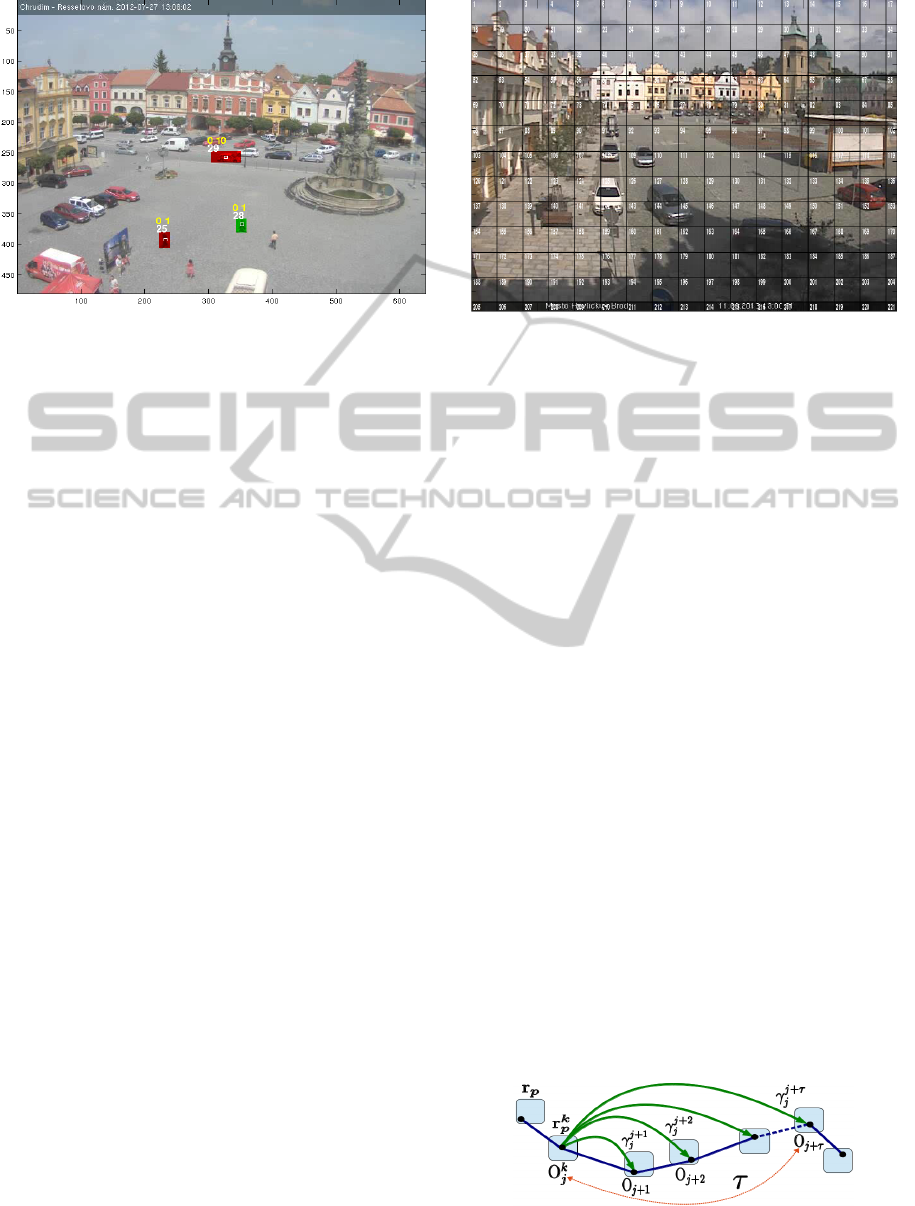
Figure 1: Sample of three objects in LOST video #1 using
labeling according to Table 2 (above and left) and Table 1
(above and right). The white number represents the track.
2.2 Scene Modeling
Our idea is to cluster data in each region where the
centroid of each object is observed. This region is a
square area with side measuring p
u
pixels which is
defined here as grid factor and p
u
∈ N
∗
. Then a fixed
grid is defined with regions having a resolution equal
to or less than the resolution of the video frame. As-
suming the resolution frame R ×C pixels, the regions
{r
p
}
g
p=1
, are numbered sequentially from left to right
and top to bottom turning the grid into a unidimen-
sional vector of regions where g = dR/p
u
e.dC/p
u
e.
In this respect, the two dimensions representing the
position of the centroid of an object is reduced to a
scalar that represents a position in the vector regions.
2.2.1 Grid Formation
The p index of the region r
p
where the object cen-
troid is located, can generically be determined by the
expression p = b(x
u
− 1)/p
u
c.dC/p
u
e + dy
u
/p
u
e, ac-
cording to the current 2D centroid position (x
u
,y
u
)
were {x
u
}
R
1
and {y
u
}
C
1
. The region defined as r
1
of
set {r
p
}
g
p=1
is the first set of pixels from the top left
of the frame. The region r
2
is immediately to the right
of r
1
and so on up to the end of the columns or rows
of the frame pixels. If C or R isn’t a multiple of the
size of p
u
, the last regions on the rigth or bottom will
have dimensions smaller than p
u
but even so, they are
labeled sequentially in the grid. Figure 2 illustrates
an example of the grid regions r
p
using a grid factor
p
u
= 39. The total area of the frame is transformed
into a one-dimensional vector with g = 221 elements.
For each frame, each object with respective 2D cen-
troid coordinates, is associated with a single region
even if the areas of the bounding box are overlapping
the neighboring regions.
Figure 2: Labeling of grid formation over a generic frame
of LOST video #17 with R ×C = 480 ×640 pixels.
2.3 Motion Modeling
Each grid region is used as a reference to store all
data vectors of a window of τ following object tran-
sitions. Obviously, the same region may belong to
other object paths, and thus, accumulating an increas-
ing amount of data. The transitions window defines
how long the track of the object should be observed.
The higher the value of τ, more specific becomes the
analysis. The assumption to be a transition is consid-
ered when an object jumped to a different region in
the next observation. Each track is observed within
the limit of the window.
The annotated dataset offers a set of n tracks T for
each video is represented as {T
k
i
}
n
i=1
and k ∈ N
∗
is
the set of frames k where the object is sampled. Each
frame k has a well defined timestamp t in the video
and t ∈ R
+
. Then T
k
i
represents a set of m observa-
tions of the same object, T
k
i
= {O
k
j
}
m
j=1
. Each obser-
vation is a set of transition vectors O
k
j
= {γ
j+a
j
}
τ
a=1
were γ
j+a
j
= (r
p
,v,t)
T
is a vector transition sampled
the trail and that contains the temporal continuous
record t (timestamp) of object type v, in region r
p
of the grid. Figure 3 shows these future transitions
observation of any object in frame k in a sampling
window up to τ. All transition vectors up to γ
j+τ
j
are
associated as samples at the region in the observation
point O
k
j
.
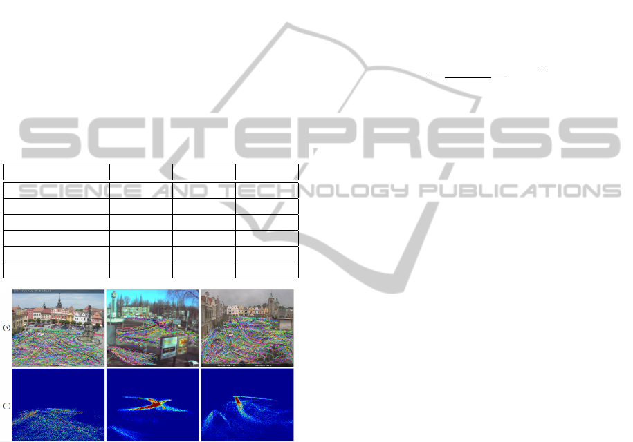
Figure 3: Detail of the motion model of a track T
i
proposed
by (Basharat et al., 2008) and adapted by us.
Region-basedAbnormalMotionDetectioninVideoSurveillance
713
2.4 Learning Modeling
To build the database for training model, it is neces-
sary the long-term observation of the scenes in order
to obtain a sufficient samples of the objects types and
their displacements. Therefore, we use three videos
with different sizes according to Table 3. The charac-
teristic of the scenarios and resolutions involved were
purposely chosen. Video #1 has a more sparse num-
ber of tracks than the others. Video #14 has most of
its tracks concentrated in specific regions of the scene.
Figure 4 shows the detail of the distribution of tracks
and samples of each video. The locations of pixels
with more intense colors are those with the largest
number of samples. The dispersion observed in sam-
ples videos #1 and #17 suggests that many areas may
have insufficient data for training of the GMM.
Table 3: Data of the video datasets corresponding values
achieved after training steps due to a factor grid p
u
= 1.
LOST dataset #1 #14 #17
resolution 480x640 240x320 480x640
hours 4 4 5
anormal tracks 37 32 116
normal tracks 1190 1755 2990
transitions 54661 58072 115688
samples 816018 777044 1646275
Figure 4: Scenarios samples used according to the LOST
datasets. In (a) video #1, video #14 and video #17, in this
order, In (b), the corresponding normalized distributions.
Any deviation of usual local or global motion, re-
sults in significant differences when calculating the
probability and abnormalities are so identified. As
an example, a person riding a motorcycle who moves
on a trajectory and speed of usual pedestrians, should
only be identified as an object with abnormal motion
if it is on a sidewalk.
An iterative process conducted in off-line mode is
done to find the value or range of values of p
u
which
leads to the best performance in the identification of
abnormal motions. In the first step of training, all
tracks annotated as abnormal, are excluded from the
dataset. The sampling for each region is performed
according motion model. Therefore, this method
refers to a supervised learning since the training data
consists of only one class normal events (Sodemann
et al., 2012). In the second step, the dataset contain
normal and abnormal events so that all tracks have an-
notations to be used as targets in lifting ROC curves.
The found threshold represents the lowest probability
of all transitions sampled in the scenario. Considering
the dimensionality of data clusters equal 3, in sum-
mary, the probability is determined through equation
(1), where η
p
represents the samples quantity in each
region r
p
and a = {1,2,...τ}.
P(γ
j−a
|(Σ,µ)
r
p
) =
1
p
(2π)
3
|Σ|η
p
exp
−
1
2
(Σ−µ)
T
Σ
−1
(Σ−µ)
(1)
In each iteration we saved into vectors, the amount
of samples used in the training steps and the threshold
value associated with the best ROC curve efficiency.
The value of p
u
is incremented by one from the uni-
tary value. After some experiments, our simulations
are stopped for the value of p
u
= 30. The limit of p
u
increment and the metric ROC efficiency is discussed
in section 3.
At the end of this process, one of the p
u
values and
respective best threshold ROC curve associated can
be adopted for the monitored scenario. The known
threshold is going to be used as a single-class classi-
fier until the necessity of another round. Since both
p
u
and respective decision threshold values is chosen,
any size or video sequence in the same video scenery
which contains the annotations on its tracking, can be
tested. One off-line round can be summarized in the
following pseudo-code:
INITIALIZATION; pumax=30; tau=20; targets;
FOR pu=1 TO pumax
\\ 1st Training Step with dataset one-class
r(p)={}: p=1 TO ALL grid regions g;
FOR all n tracks in each j transition
JOIN in r(j+a),[r(j),v(j),t(a-j)],a=1:tau;
FOR p=1 to g
RUN EM over Gaussian Mixtures in r(p);
SAVE learned parameters sigma_p,mu_p,k_p;
END
END
\\ 2nd Training Step with full dataset
FOR all n tracks in each j transition
out_n = estimate min probability in r(j)|p
from tau previous transitions;
END
RUN ROC curve from (out,targets)_n vector;
threshold_n=ROC efficiency metric;
PLOT samples_used and threshold_n by pu;
END
FIND best(pu,threshold) ranges among all plots;
END
ICPRAM2014-InternationalConferenceonPatternRecognitionApplicationsandMethods
714
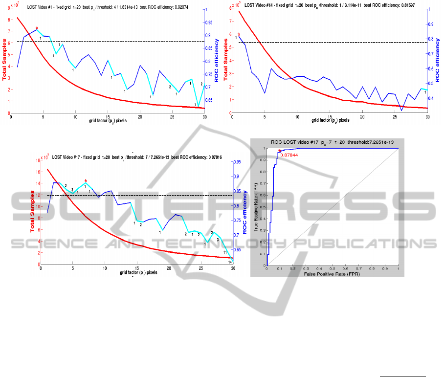
(a) video #1. (b) video #14.
(c) video #17. (d) Best ROC curve of video #17.
Figure 5: Effects of the increased grid factor over the amount of samples and the performance in abnormal motion detection.
On a test model, for each new position of each
object in each frame and using equation (1), it is esti-
mated the probability of that type of object to be at the
current position and time, originating from each of the
τ previous transitions (high order analysis). If any of
the τ probabilities is less than the used threshold, then
the object is identified as describing an unusual tra-
jectory from that point until the end of its trajectory
tracking in video. In our implementation, we high-
light in red color the bounding box of the object that
had its motion identified as abnormal.
3 RESULTS
In the context of this work, we have compiled the
main data results through the curves shown in Fig-
ure 5. The curves show the relationship between the
number of involved samples (red curves) and the ROC
efficiency metric for each p
u
value. For them, a tran-
sition windows τ = 20 was adopted.
Since we are only interested in the highest hit
rate of true positives (T PR) and the lowest hit rate of
false positives (FPR), we adopted as reference met-
ric the ROC efficiency through equation 2. (Powers,
2011) suggests a goodness performance measure for
(T PR −FPR), called informedness. A number closer
to 1, indicates better correct ratio for both abnormal
and the normal tracks. The value of ε represents the
number of lost tracks, which is explained hereafter.
ROCe f f iciency = (T PR − FPR).(1 −
ε
total tracks
)
2
(2)
As an example, the curve in Figure 5(c) shows that
the best ROC efficiency value occurs when p
u
= 7.
The asterisk character presents the best outcome of
the equation 2. Figure 5(d) shows the detail of best
ROC curve and corresponding threshold value.
The numbers alongside different color segments
plotted in the ROC efficiency curve, represent the
amount of tracks that have been lost for two reasons:
(i) the number of samples in all object transition re-
gions wasn’t enough for the convergence of the GMM
training algorithm (usually the clusters require at least
30 samples) and (ii) lack of transitions between re-
gions. In our tests, the hypothesis (i) was most rep-
resentative. These losses are well demonstrated in
videos #1 and #17 due to fact that they have a sam-
ple dispersion in many regions of interest, as shown
in Figure 4 (b). The hypothesis (ii) becomes relevant
for larger p
u
values. Higher values of p
u
decreases
the transitions amounts. These larger regions can con-
Region-basedAbnormalMotionDetectioninVideoSurveillance
715

tain most or all samples of a shorter track. This was
the reason why we adopt the limit p
u
= 30, because
from that value on, the loss of tracks get larger. When
tracks are lost, they affect TPR and FPR ratios and
become unequal in results comparison. To avoid this
negative influence, we apply a penalty factor accord-
ing to equation (2) which takes into consideration the
loss of ε tracks in relation to the total tracks.
We consider an optimal range of grid factors p
u
for each LOST video. This range must have a min-
imum track loss and must not be less than the value
when p
u
= 1. The boundary of this range in Fig-
ure 5 is represented by the horizontal dashed line. It
is also clear that in all tested videos there is a com-
mon performance improvement when 1 . p
u
. 10.
In this range, the number of samples decreases up to
∼60% if compared with equivalent pixel-based mod-
els (when p
u
= 1). This is the case of video #17 were
the number of samples starts in ∼1.64 milion when
p
u
= 1 and decreases to 648,483 when p
u
= 9.
If we extend the comparison with the previous ap-
proach presented by (Basharat et al., 2008), the dif-
ference is huge due to the motion model these au-
thors makes sample copies in all pixels of bounding
box boundary. In a simulation using the dataset avail-
able by the authors, with video resolution 240x320
pixels and ∼3 hours length, we observed more than
250 million samples and the ROC curve with much
lower performance than we present in Figure 5(d).
The training time was dependent on the video ac-
cording to the samples concentration per region. So,
considering the best value of p
u
, all videos had their
training time much lower than total time of the videos.
The input vector for the space-time motion model
is reduced to a 3-dimensional space with (r
p
,v,t). The
distribution of the data vectors in hyperplanes tends to
be sparse. This harms the accuracy and convergence
of the GMM models. Otherwise, too many samples,
or oversampling form a lot of less representative clus-
ters which require more unnecessary computational
effort. In videos #1 and #17 it is notable the fast ef-
ficiency increasing from p
u
= 1. This is an expected
effect because the increasing of regions area, samples
will be adding in these regions and help to ensure or to
improve the clusters during GMM training. This be-
havior isn’t observed with video #14 due to the higher
concentration of samples in a small area in the cen-
ter of the video even when p
u
= 1 (see detail in Fig-
ure 4 (b)). When p
u
> 1 an oversampling occurs and
this saturation has not produced good results in the
GMM training. The behavior leads to the conclusion
that region-based models do not require many sam-
ples, however they need to be better distributed.
4 FURTHER WORKS
The method has shown insensitivity to scene context
and low dependency on the robustness of the tracking
algorithm. The uniform behavior of the performance
curves revels these tendency, since they deal with dif-
ferent resolutions, areas of interest, object’s bounding
box fidelity and their tracking, number of track tran-
sitions, number of tracks and video length. In this
aspect, the LOST project opens opportunities for re-
search in scene analysis involving long-term surveil-
lance in outdoor environments. We intend to use it
also for future studies, including the application of the
same method presented here, but using others statisti-
cal models such as HMM.
We observe that the p
u
range values which leads
to the best performance of the method, tend to match
with the smallest object size tracked (high or width).
These information did not explicitly participate in the
training. Currently, we are engaged in evidence and
theoretical explanation of this trend.
We intend to continue the study of this approach
using a mobile grid rather than a fixed one, as well as
using algorithms like superpixel segmentation.
Alternatively, since the computational effort is re-
duced due to the lower amount of samples, it is possi-
ble to keep a training window in on-line mode. Sim-
ply replacing old samples and repeating the GMM
model training only for updated regions.
5 CONCLUSIONS
We present a new method for abnormal motion de-
tection in real video surveillance scenes. We comple-
mented with video annotations the preexisting tracks
of the LOST dataset. The proposed region-based
method supported by ROC curves, used scene, mo-
tion and learning models focused on dimensionality
reduction to decrease the computational effort with-
out sacrificing performance in detecting abnormali-
ties. Our method avoids the excessive data and so-
phisticated algorithms used in many pixel-based ap-
proaches. In addition, appearance models of objects
did not need to be defined, like most of the region-
based strategies.
Our results show that the method is useful and also
shown good behavior for different scenarios, contexts,
quantity and quality of samples. They have demon-
strated that there is a range of grid factor values that
maintain the efficiency in motion analysis, even with
a significant reduction in the number of samples used
to train a statistical model such as the GMM.
ICPRAM2014-InternationalConferenceonPatternRecognitionApplicationsandMethods
716

REFERENCES
Abrams, A., Tucek, J., Little, J., Jacobs, N., and Pless, R.
(2012). LOST: Longterm Observation of Scenes (with
Tracks). In Applications of Computer Vision (WACV),
2012 IEEE Workshop on, pages 297–304.
Basharat, A., Gritai, A., and Shah, M. (2008). Learning
object motion patterns for anomaly detection and im-
proved object detection. In Computer Vision and Pat-
tern Recognition, 2008. CVPR 2008. IEEE Confer-
ence on, pages 1–8.
Berclaz, J., Fleuret, F., and Fua, P. (2008). Multi-camera
Tracking and Atypical Motion Detection with Behav-
ioral Maps. In ECCV (3), pages 112–125.
Bishop, C. M. (2006). Pattern Recognition and Machine
Learning. Springer, New York.
Cong, Y., Yuan, J., and Tang, Y. (2013). Video Anomaly
Search in Crowded Scenes via Spatio-Temporal Mo-
tion Context. IEEE Transactions on Information
Forensics and Security, 8(10):1590–1599.
Elhoseiny, M., Bakry, A., and Elgammal, A. (2013). Multi-
Class Object Classication in Video Surveillance Sys-
tems Experimental Study. In CVPR’13, pages 788–
793.
Ermis, E. B., Saligrama, V., Jodoin, P.-M., and Konrad, J.
(2008). Motion segmentation and abnormal behavior
detection via behavior clustering. In ICIP, pages 769–
772. IEEE.
Feizi, A., Aghagolzadeh, A., and Seyedarabi, H. (2012).
Behavior recognition and anomaly behavior detection
using clustering. In Telecommunications (IST), 2012
Sixth International Symposium on, pages 892–896.
Figueiredo, M. A. T. and Jain, A. (2002). Unsupervised
learning of finite mixture models. Pattern Analy-
sis and Machine Intelligence, IEEE Transactions on,
24(3):381–396.
Hanapiah, F., Al-Obaidi, A., and Chan, C. S. (2010).
Anomalous trajectory detection using the fusion of
fuzzy rule and local regression analysis. In Infor-
mation Sciences Signal Processing and their Applica-
tions (ISSPA), 2010 10th International Conference on,
pages 165–168.
Haque, M. and Murshed, M. (2012). Abnormal Event De-
tection in Unseen Scenarios. In Multimedia and Expo
Workshops (ICMEW), 2012 IEEE International Con-
ference on, pages 378–383.
Jiang, F., Yuan, J., Tsaftaris, S. A., and Katsaggelos, A. K.
(2011). Anomalous video event detection using spa-
tiotemporal context. Computer Vision and Image Un-
derstanding, 115(3):323–333.
Kiryati, N., Riklin-Raviv, T., Ivanchenko, Y., and Rochel,
S. (2008). Real-time abnormal motion detection in
surveillance video. In ICPR, pages 1–4. IEEE.
Kwon, E., Noh, S., Jeon, M., and Shim, D. (2013). Scene
Modeling-Based Anomaly Detection for Intelligent
Transport System. In Intelligent Systems Modelling
Simulation (ISMS), 2013 4th International Confer-
ence on, pages 252–257.
Li, H., Achim, A., and Bull, D. (2012). Unsupervised video
anomaly detection using feature clustering. Signal
Processing, IET, 6(5):521–533.
Oh, S., Hoogs, A., Perera, A. G. A., Cuntoor, N. P., Chen,
C.-C., Lee, J. T., Mukherjee, S., Aggarwal, J. K., Lee,
H., Davis, L. S., Swears, E., Wang, X., Ji, Q., Reddy,
K. K., Shah, M., Vondrick, C., Pirsiavash, H., Ra-
manan, D., Yuen, J., Torralba, A., Song, B., Fong, A.,
Chowdhury, A. K. R., and Desai, M. (2011). AVSS
2011 demo session: A large-scale benchmark dataset
for event recognition in surveillance video. In AVSS,
pages 527–528. IEEE Computer Society.
Powers, D. M. W. (2011). Evaluation: From Precision, Re-
call and F-Factor to ROC: Informedness, Markedness
& Correlation. Journal of Machine Learning Tech-
nologies, 2(Issue 1):37–63.
R
¨
aty, T. (2010). Survey on Contemporary Remote Surveil-
lance Systems for Public Safety. Systems, Man, and
Cybernetics, Part C: Applications and Reviews, IEEE
Transactions on, 40(5):493–515.
Shi, Y., 0001, Y. G., and Wang, R. (2010). Real-Time Ab-
normal Event Detection in Complicated Scenes. In
ICPR, pages 3653–3656. IEEE.
Sodemann, A. A., Ross, M. P., and Borghetti, B. J.
(2012). A Review of Anomaly Detection in Auto-
mated Surveillance. IEEE Transactions on Systems,
Man, and Cybernetics, Part C, 42(6):1257–1272.
Tziakos, I., Cavallaro, A., and Xu, L.-Q. (2010). Local Ab-
normality Detection in Video Using Subspace Learn-
ing. In Advanced Video and Signal Based Surveillance
(AVSS), 2010 Seventh IEEE International Conference
on, pages 519–525.
Zeng, S. and Chen, Y. (2011). Online-learned classifiers
for robust multitarget tracking. In Neural Networks
(IJCNN), The 2011 International Joint Conference on,
pages 1275–1280.
Region-basedAbnormalMotionDetectioninVideoSurveillance
717
