A Semi-Lagrangian Approximation of the Oren–Nayar PDE
for the Orthographic Shape–from–Shading Problem
Silvia Tozza and Maurizio Falcone
Department of Mathematics, Sapienza - Universit
`
a di Roma, P.le Aldo Moro 5, Rome, Italy
Keywords:
Shape–from–Shading, Oren–Nayar Differential Model, Semi-Lagrangian Approximation Scheme.
Abstract:
Several advances have been made in the last ten years to improve the Shape–from–Shading model in order to
allow its use on real images. The classic Lambertian model, suitable to reconstruct 3D surfaces with uniform
reflection properties has shown to be unsuitable for other types of surfaces, for example for rough objects
consisting of materials such as clay. Other models have been proposed but it is still unclear what would be
the best model. For this reason, we start our analysis for non-Lambertian surfaces. The goal being to find a
unique model which should be flexible enough to deal with many kinds of real images. As a starting point for
this big project, we consider the non-Lambertian Oren–Nayar reflectance model. In this paper we construct
a semi-Lagrangian approximation scheme for its nonlinear partial differential equation and we compare its
performances with the classical model in terms of some error indicators on series of benchmarks images.
1 INTRODUCTION
The Shape–from–Shading (SfS) problem is a classical
inverse problem in Computer Vision: given a bidi-
mensional image, the goal is to compute the three-
dimensional shape of the surface from the brightness
of one gray level image of that surface. The literature
of this problem is huge as one see looking at the refer-
ences in the survey papers (Zhang et al., 1999; Durou
et al., 2008). However, the large majority of these
contribution have addressed the case of Lambertian
surfaces improving the model with the introduction
of perspective deformations (Courteille et al., 2004;
Prados et al., 2006; Breuß et al., 2012), studying sev-
eral techniques to obtain a numerical approximation
of the variational problem (Horn and Brooks, 1986)
and of the corresponding differential model (Lions
et al., 1993) or studying the corresponding photo-
metric stereo problem (Onn and Bruckstein, 1990;
Mecca and Falcone, 2013). We focus our attention
on a different improvement which is intended to re-
duce the assumptions on the properties of the surface
dealing with more general (and real) non-Lambertian
surfaces. Our goal is to find a unique model which
should be flexible enough to handle many different
kinds of real images. To this end we want to an-
alyze in a unified framework several models which
have been proposed in the literature, e.g. (Phong,
1975; Oren and Nayar, 1995). As a starting point for
this rather big project, we consider the basic model of
a single nonlinear partial differential equation (PDE)
where we need to introduce new terms to tackle the
general non-Lambertian case. In particular, here we
consider the non-Lambertian Oren–Nayar reflectance
model proposed in (Oren and Nayar, 1994; Oren and
Nayar, 1995), we construct a semi-Lagrangian ap-
proximation scheme for its nonlinear PDE and we
compare its performances with the classical model.
Other models will be studied in a forthcoming paper
(Falcone and Tozza, 2014) where we will also com-
pare different approaches.
2 TWO SfS MODELS
In order to underline the differences, let us briefly
sketch the classical Lambertian model (L–model) and
the Oren–Nayar model (ON–model).
Let us consider a surface given as a graph z =
u(x),x ∈ R
2
. We assume that u(x) ≥ 0 and the sur-
face is standing on a flat background, we will denote
by Ω the region inside the silhouette and we will as-
sume (just for technical reasons) that Ω is an open and
bounded subset of R
2
. Moreover, we consider a single
light source located at infinity. It is well known that
the SfS problem is described by the image irradiance
equation
I(x) = R(N(x)), (1)
711
Tozza S. and Falcone M..
A Semi-Lagrangian Approximation of the Oren–Nayar PDE for the Orthographic Shape–from–Shading Problem.
DOI: 10.5220/0004855007110716
In Proceedings of the 9th International Conference on Computer Vision Theory and Applications (VISAPP-2014), pages 711-716
ISBN: 978-989-758-009-3
Copyright
c
 2014 SCITEPRESS (Science and Technology Publications, Lda.)

where I(x) is the normalized brightness of the given
grey-value image, N(x) is the unit normal to the sur-
face at the point (x,u(x)) and R(N(x)) is the reflection
map giving the value of the light reflection on the sur-
face as a function of its orientation (i.e., of the normal)
at each point. For a Lambertian surface the irradiance
equation becomes I(x) = γ N ·ω, where we assume to
know the albedo gamma (in the sequel we put γ = 1
for simplicity). For Lambertian surfaces (Horn and
Brooks, 1986; Horn and Brooks, 1989), just consider-
ing an orthographic projection of the scene, it is pos-
sible to model the SfS problem via a nonlinear PDE
of the first order which describes the relation between
the surface u (our unknown) and the brightness func-
tion I. In fact, recalling that the normal to a graph is
given by N(x) = (−u
x
1
,−u
x
2
,1)/
p
1 + |∇u(x)|
2
, we
can write (1) as
I(x)
q
1 + |∇u(x)|
2
+
e
ω ·∇u(x) −ω
3
= 0, in Ω (2)
where
e
ω = (ω
1
,ω
2
). This is an Hamilton-Jacobi type
equation which does not admit in general regular so-
lution. It is known that the mathematical framework
to describe its weak solutions is the theory of viscos-
ity solutions as in (Lions et al., 1993). For analytical
and numerical reasons it is useful to introduce the ex-
ponential transform µv(x) = 1 −e
−µu(x)
and change
the variable. Note that here µ is a free positive param-
eter without a physical meaning. Following (Falcone
et al., 2003), we can write (2) in a fixed point form





µv(x) = min
a∈∂B
3
{b(x,a) ·∇v(x) + f (x,a,v(x))}
for x ∈ Ω,
v(x) = 0 for x ∈ ∂Ω.
(3)
where b(x,a) =
1
ω
3
(I(x)a
1
−ω
1
,I(x)a
2
−ω
2
),
f (x,a,v(x)) = −
I(x)a
3
ω
3
(1 −µv(x))}+ 1 and B
3
is the
unit ball in R
3
.
In contrast to the standard Lambertian case that as-
sumes the object surface to be ideally diffusive, the
ON–model (Oren and Nayar, 1994; Oren and Nayar,
1995) explicitly allows to handle rough surfaces. The
idea of this model is to represent a rough surface as an
aggregation of V-shaped cavities, each with Lamber-
tian reflectance properties (see Fig. 1). The bright-
V-cavity
facet
dA
Figure 1: Facet model for surface patch dA consisting of
many V-shaped Lambertian cavities.
ness equation for the ON–model is given by
I(x) = cos(θ
i
)A + Bsin(α)tan(β)M(ϕ
i
,ϕ
r
) (4)
where
M(ϕ
i
,ϕ
r
) = max[0,cos(ϕ
i
−ϕ
r
)] (5)
A = 1 −0.5 σ
2
(σ
2
+ 0.33)
−1
(6)
B = 0.45σ
2
(σ
2
+ 0.09)
−1
. (7)
Note that A and B are two nonnegative constants de-
pending on the statistics of the cavities via the rough-
ness parameter σ. In this model, θ
i
represents the an-
gle between the unit surface normal N and the light
source direction ω, θ
r
stands for the angle between the
unit surface normal N and the camera direction V, ϕ
i
is the angle between the projection of the light source
direction ω and the x
1
axis onto the (x
1
,x
2
)-plane, ϕ
r
denotes the angle between the projection of the cam-
era direction V and the x
1
axis onto the (x
1
,x
2
)-plane
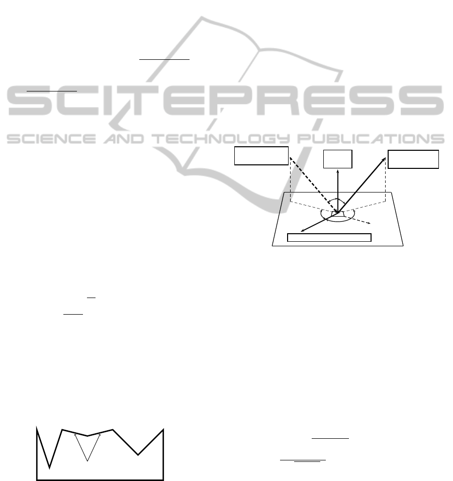
(see Fig. 2), and the two variables α and β are given
by
α = max[θ
i
,θ
r
] and β = min [θ
i
,θ
r
]. (8)
Surface
normal
Camera:
reflected light (I)
Point l ight source:
incident light (L
i
)
φ
r
−φ
i
θ
r
θ
i
Reference direction on the surface
dA
Figure 2: Diffuse reflectance for the ON–model.
For smooth surfaces, we have σ = 0 and the ON–
model brings back to the L–model. To deal with this
equation one has to resolve the min and max opera-
tors which appear in (4), (8). In general, some cases
must be considered but here we just take one to il-
lustrate the technique. Namely, we consider the par-
ticular case where the position of the light source ω
coincides with the camera direction V. This choice
implies max[0, cos(ϕ
i
−ϕ
r
)] = 1, then defining θ :=
θ
i
= θ
r
= α = β, the equation (4) simplifies to
I(x) = cos(θ)

A+B sin(θ)
2
cos(θ)
−1

(9)
and we arrive to a Dirichlet problem for the first order
nonlinear Hamilton-Jacobi equation







(I(x) −B)(
p
1 + |∇u|
2
) + A(
e
ω ·∇u −ω
3
)
+B
(−
e
ω·∇u+ω
3
)
2
√
1+|∇u|
2
= 0, x ∈ Ω,
u(x) = 0 x ∈ ∂Ω,
(10)
where
e
ω = (ω
1
,ω
2
). Note that the simple homo-
geneous Dirichlet boundary condition is due to the
VISAPP2014-InternationalConferenceonComputerVisionTheoryandApplications
712

flat background behind the object but a condition like
u(x) = g(x) can also be considered if necessary.
Following (Falcone et al., 2003), we write the sur-
face as S(x,z) = z −u(x) = 0, for x ∈ Ω, z ∈ R, and
∇S(x,z) = (−∇u(x), 1), (10) becomes







(I(x) −B)|∇S(x,z)|+ A(−∇S(x,z) ·ω)
+B

∇S(x,z)
|∇S(x,z)|
·ω

2
|∇S(x,z)| = 0, x ∈Ω,
u(x) = 0 x ∈ ∂Ω.
(11)
Defining d(x,z) = ∇S(x,z)/|∇S(x,z)| and c(x,z) =
I(x) − B + B(d(x, z) · ω)
2
, using the equivalence
|∇S(x,z)| ≡ max
a∈∂B
3
{a ·∇S(x,z)} we get
max
a∈∂B
3
{c(x,z)a ·∇S(x,z) −Aω ·∇S(x, z)} = 0. (12)
Defining the vectorfield
b
ON
(x,a) =
1
Aω
3
(c
1
(x,z)a
1
−Aω
1
,c
2
(x,z)a
2
−Aω
2
) (13)
we can finally write the nonlinear equation corre-
sponding to the ON–model,





µv(x) + max
a∈∂B
3
{−b
ON
(x,a) ·∇v(x)
+
c
3
(x,z)a
3
Aω
3
(1 −µv(x))} = 1, x ∈ Ω,
v(x) = 0 x ∈ ∂Ω.
(14)
3 SEMI-LAGRANGIAN
APPROXIMATION SCHEMES
The numerical schemes used in this paper are based
on a semi-Lagrangian approach. This method has
shown to be very effective for first order problems
since it tries to mimic at the discrete level the method
of characteristics (see (Falcone and Ferretti, 2013) for
more details). Let W
i
= w(x
i
) so that W will be the
vector solution giving the approximation of the height
of u at every node x
i
of the grid. The fully discrete
scheme for the classical L–model is given by
W
i
= T
i
(W ). (15)
Denoting by P the global number of nodes in the grid,
the operator T : R
P
→ R
P
is defined componentwise
by
T
i
(W ) = min
a∈∂B
3
{e
−µh
w(x
i
+ hb(x
i
,a))
−τ
I(x
i
)a
3
ω
3
(1 −µw(x
i
))}+ τ,
(16)
where τ = 1 −e
−µh
/µ and w(x
i
+ hb(x
i
,a)) is ob-
tained interpolating on W .
It has been shown in (Falcone et al., 2003) that the
corresponding operator T has three important prop-
erties: it is monotone, is a contraction mapping in
[0,1/µ)
P
and 0 ≤W ≤
1
µ
implies 0 ≤ T (W ) ≤
1
µ
.
Similarly, the SL fully discrete scheme for the ON–
model at a node x
i
is given by
W
i
= T
ON
i
(W ) (17)
where the discrete operator T
ON
is defined as
T
ON
i
(W ) = min
a∈∂B
3
{e
−µh
w(x
i
+ hb
ON
(x
i
,a))
−τ
c
3
(x
i
,z)a
3
Aω
3
(1 −µw(x
i
))}+ τ.
(18)
The proof of the properties of the operator T
ON
will
appear in (Falcone and Tozza, 2014).
4 NUMERICAL TESTS
In this section we show some numerical tests to com-
pare the two schemes described in the previous sec-
tion. The algorithm for both the schemes is based on
the fixed-point iteration

V
n
= T (V
n−1
),
V
0
given.
(19)
For the ON–model T is clearly replaced by T
ON
.
For the synthetic images, we discretize the domain
Q with 151×151 nodes. The fixed point has been
computed with an accuracy of η = 10
−4
and the
stopping rule used is max(|V
n+1
−V
n
|) ≤ η.
The first experiment is related to the paraboloid
in [−1.5,1.5]x[−1.5,1.5] described by the function
z(x,y) =

1 −(x
2
+ y
2
) if (x
2
+ y
2
) < 1,
0 otherwise,
(20)
with light direction ω = (0,0,1) and visible in Fig. 3.
Figure 3: Test 1: Original surface u(x,y).
As one can see in Fig. 4, there are no significant
differences between the two surfaces reconstructed,
but we can note from Tables 1, 2 and 3 that increas-
ing of the value of the roughness parameter σ the er-
ror generated by the method of Oren–Nayar decreases
ASemi-LagrangianApproximationoftheOren-NayarPDEfortheOrthographicShape-from-ShadingProblem
713

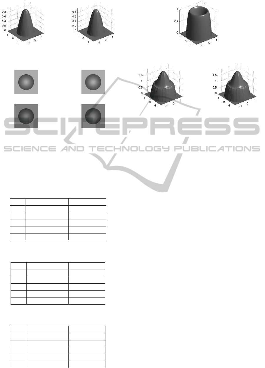
Figure 4: Test 1: Surface reconstruction, L–model (left) and
ON–model with σ = 0.8 (right).
I(x) phong
I(x) approssimata Phong
Input I(x) Computed I(x)
Input I(x) Computed I(x)
Figure 5: Test 1: Images, ON–model with σ = 0.8 (up) and
L–model (down).
and it is lower than the error for the L–model. Note
that for σ = 0 we get exactly the same result (since
the two models coincide). In Fig. 5 the background
gray level is different because it has been computed
via the model.
Table 1: Test 1: L
∞
Error on the image with respect to σ.
σ L
∞
Error Lamb L
∞
Error ON
0 0.074826 0.074826
0.3 0.074826 0.066809
0.5 0.074826 0.058700
0.8 0.074826 0.050141
π/2 0.074826 0.041826
Table 2: Test 1: L
1
Error on the image for different values
of σ.
σ L
1
Error Lamb L
1
Error ON
0 0.028256 0.028256
0.3 0.028256 0.025228
0.5 0.028256 0.022166
0.8 0.028256 0.018934
π/2 0.028256 0.015795
Table 3: Test 1: Standard Deviation on the image for differ-
ent values of σ.
σ Std Dev. Lamb Std Dev. ON
0 0.007426 0.007426
0.3 0.007426 0.006631
0.5 0.007426 0.005826
0.8 0.007426 0.004976
π/2 0.007426 0.004151
Figure 6: Test 2: Original surface u(x,y).
Figure 7: Test 2: Approximated surface u(x,y) with the two
schemes that compute the maximal viscosity solution.
The second numerical test is related to the surface
described by the function
z(x,y) =

−(1 −(x
2
−y
2
))
2
+ 1 if (x
2
+ y
2
) < 2,
0 otherwise,
(21)
with light direction ω = (0,0,1) in the same domain
of the previous test (See Fig. 6 for the input surface).
Looking at Fig. 7 we can note that both the schemes
choose the maximal viscosity solution, which does
not coincide with the original surface. In order to
obtain a reconstruction closer to the original surface,
we fix the value in the origin at zero. In this way
we forced schemes to converge to a solution different
from the maximal one (see Fig. 8). Also in this case
we can see that the reconstruction of the surface is
very similar with the two schemes. In Fig. 9 note that
the background gray level is different for the same
reason of the Fig. 5.
The next test is on a real-world image: the bust
of Beethoven (see Fig. 10). The light direction is
ω = (−0.19798,−0.01680, 0.98006) and the size of
the input image is 77×210. Obviously, in the case of
real image, not all the values for σ are possible be-
cause the input image is given. After finding a correct
value for the parameter σ, we can see again in Fig. 10
that the approximations generated by the two schemes
are more o less the same, but the values in Tables 4, 5
and 6 show that the different error on the image with
the ON–model are lower than the errors obtained with
the L–model. Note that the improvement is more evi-
dent in Table 6.
The last test concerns the reconstruction of a vase
enlightened by a vertical light source. The size of the
input image is 128×128. We can see in Fig. 11 the ap-
proximated images with the two schemes on the right,
VISAPP2014-InternationalConferenceonComputerVisionTheoryandApplications
714

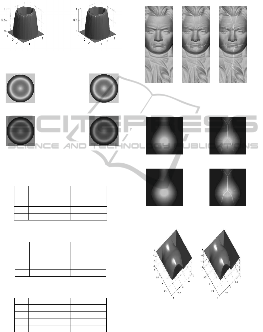
Figure 8: Test 2: Approximated surface u(x, y), L–model
(left) and ON–model (right).
I(x) phong
I(x) approssimata Phong
Input I(x) Computed I(x)
Input I(x) Computed I(x)
Figure 9: Test 2: Images, ON–model with σ = 0.5 (up) and
L–model (down).
Table 4: L
∞
Error on the image with L–model and ON–
model related to the Beethoven Test.
σ L
∞
Error Lamb L
∞
Error ON
0 0.635977 0.635977
0.2 0.635977 0.567406
0.4 0.635977 0.515963
0.5 0.635977 0.419684
Table 5: L
1
Error on the image with L–model and ON–
model related to the Beethoven Test.
σ L
1
Error Lamb L
1
Error ON
0 0.047027 0.047027
0.2 0.047027 0.045838
0.4 0.047027 0.043205
0.5 0.047027 0.042169
Table 6: Standard deviation on the image with L–model and
ON–model related to the Beethoven Test.
σ Std Dev. Lamb Std Dev. ON
0 0.056253 0.056253
0.2 0.056253 0.054361
0.4 0.056253 0.050138
0.5 0.056253 0.048308
starting from the same input image on the left. The
reconstructed surface computed by both methods is
shown in Fig. 12. As in the previous real test, the
L
∞
and the L
1
errors obtained with the Oren–Nayar
Input I(x)
a)
Computed I(x)
b)
Computed I(x)
c)
Figure 10: a) Beethoven input image. b) Oren–Nayar com-
puted image with σ = 0.4. c) Lambertian computed image.
Input I(x) Computed I(x)
Input I(x) Computed I(x)
Figure 11: Vase images: ON–model with σ = 0.4 (up) and
L–model (down).
Figure 12: Vase reconstruction: L–model (left) and ON–
model (right).
approach are always lower than the Lambertian errors
how we can note looking at the Table 7 and 8.
Our program is to proceed in the analysis of more
complex cases, e.g. synthetic images obtained with an
oblique light direction, to verify that the ON-model
is better than the classical L-model and to quantify
ASemi-LagrangianApproximationoftheOren-NayarPDEfortheOrthographicShape-from-ShadingProblem
715

Table 7: L
∞
Error on the image with L–model and ON–
model related to the vase Test.
σ L
∞
Error Lamb L
∞
Error ON
0 0.808202 0.808202
0.2 0.808202 0.766265
0.4 0.808202 0.678274
0.5 0.808202 0.634672
Table 8: L
1
Error on the image with L–model and ON–
model related to the vase Test.
σ L
1
Error Lamb L
1
Error ON
0 0.028919 0.028919
0.2 0.028919 0.027292
0.4 0.028919 0.023764
0.5 0.028919 0.022190
the differences in terms of computational complexity
and accuracy. We also plan to compare the results for
the orthographic projection and the perspective pro-
jection model introduced in (Ju et al., 2013).
5 CONCLUSIONS
The non-Lambertian models lead to rather complex
nonlinear PDEs of the first order which can be treated
in the framework of weak (viscosity) solutions. The
analysis of this models shows that they are not able
to resolve the well known convex/concave ambigu-
ity despite the fact that they can deal with more gen-
eral surfaces. From the numerical point of view, these
equations can be approximated via semi-Lagrangian
techniques in a rather effective way. The role of the
roughness parameter σ is crucial to obtain accurate
results, playing with this parameter can in fact im-
prove the approximation with respect to the classical
L–model. In this respect, the non-Lambertian frame-
work is more flexible and effective.
REFERENCES
Breuß, M., Cristiani, E., Durou, J.-D., Falcone, M., and Vo-
gel, O. (2012). Perspective shape from shading: Am-
biguity analysis and numerical approximations. SIAM
J. Imaging Sciences, 5(1):311–342.
Courteille, F., Crouzil, A., Durou, J. D., and Gurdjos, P.
(2004). Towards shape from shading under realistic
photographic conditions. 17th International Confer-
ence on Parttern Recognition, pages 277–280.
Durou, J., Falcone, M., and Sagona, M. (2008). Numerical
methods for shape from shading: a new survey with
benchmarks computer vision and image understand-
ing. Elsevier, 109(1):22–43.
Falcone, M. and Ferretti, R. (2013). Semi-Lagrangian Ap-
proximation Schemes for Linear and Hamilton-Jacobi
Equations. SIAM.
Falcone, M., Sagona, M., and Seghini, A. (2003). A scheme
for the shape-from-shading model with ”black shad-
ows”. In Numerical Mathematics and Advanced Ap-
plications. Springer-Verlag.
Falcone, M. and Tozza, S. (2014). Analysis and approxi-
mation of some Shape–from-Shading models for non-
lambertian surfaces. Forthcoming.
Horn, B. and Brooks, M. (1986). The variational approach
to shape from shading. Computer Vision, Graphics,
and Image Processing, 33(2):174–208.
Horn, B. and Brooks, M. (1989). Shape from Shading. The
MIT Press.
Ju, Y. C., Tozza, S., Breuß, M., Bruhn, A., and Kleefeld,
A. (2013). Generalised Perspective Shape from Shad-
ing with Oren-Nayar Reflectance. In Proceedings of
the 24th British Machine Vision Conference (BMVC
2013), Bristol, UK. BMVA, BMVA Press.
Lions, P. L., Rouy, E., and Tourin, A. (1993). Shape-from-
shading, viscosity solutions and edges. Numerische
Mathematik, 64(3):323–353.
Mecca, R. and Falcone, M. (2013). Uniqueness and approx-
imation of a photometric shape-from-shading model.
SIAM J., 6(1):616–659.
Onn, R. and Bruckstein, A. M. (1990). Integrability dis-
ambiguates surface recovery in two-image photomet-
ric stereo. International Journal of Computer Vision,
5(1):105–113.
Oren, M. and Nayar, S. (1994). Generalization of Lambert’s
reflectance model. In Proc. International Conference
and Exhibition on Computer Graphics and Interactive
Techniques (SIGGRAPH), pages 239–246.
Oren, M. and Nayar, S. (1995). Generalization of the Lam-
bertian model and implications for machine vision. In-
ternational Journal of Computer Vision, 14(3):227–
251.
Phong, B. (1975). Illumination for computer generated pic-
tures. Communications of the ACM, 18(6):311–317.
Prados, E., Camilli, F., and Faugeras, O. (2006). A viscosity
solution method for shape-from-shading without im-
age boundary data. ESAIM: Mathematical Modelling
and Numerical Analysis, 40(2):393–412.
Zhang, R., Tsai, P.-S., Cryer, J., and Shah, M. (1999). Shape
from shading: a survey. IEEE Transactions on Pattern
Analysis and Machine Intelligence, 21(8):690–706.
VISAPP2014-InternationalConferenceonComputerVisionTheoryandApplications
716