
Managing Price Risk for an Oil and Gas Company
António Quintino
1,2
, João Carlos Lourenço
1
and Margarida Catalão-Lopes
1
1
CEG-IST, Instituto Superior Técnico, Universidade de Lisboa, Lisbon, Portugal
2
Galp Energia, Refining and Distribution Risk Dept., Lisbon, Portugal
Keywords: Portfolio Hedging, Risk Tolerance, Multi-criteria Decision Analysis.
Abstract: Oil and gas companies’ earnings are heavily affected by fuels price fluctuations. The use of hedging tactics
independently by each of their business units (e.g. crude oil production, oil refining and natural gas) is
widespread to diminish their exposure to prices volatility. How much should be hedged and which
derivatives should be selected according to the company risk profile are the main questions this paper
intends to answer. The present research formulates an oil and gas company’s integrated earnings structure
and evaluates the company’s risk tolerance with four approaches: Howard’s, Delquie’s, CAPM and a risk
assessment questionnaire. Stochastic optimization and Monte Carlo simulation with a Copula-GARCH
modelling of crude oil, distillates and natural gas prices is used to find the derivatives portfolios according
to company risk tolerance hypothesis. The hedging results are then evaluated with a multi-criteria model
built in accordance with the expressed company’s representatives preferences upon four criteria: payout
exposure; downside gains; upside gains; and risk premium. The multi-criteria analysis revealed a decisive
role in the final hedging decision.
1 INTRODUCTION
Oil and gas (O&G) companies’ earnings are
substantially affected by the price fluctuations of
crude oil, natural gas and refined products, which
induce these companies to find ways to minimize
price risk exposure. Almost all O&G companies use
derivative instruments, like swaps and options, to
share price risks with other counterparties. This
research intends to propose a methodology to help
answer the main question that an O&G company
faces when trying to meet its budget goals: which
amount (if any) should be hedged and in which
derivatives. This work does not intend to be an
intensive research on complex derivatives but
instead evaluates the robustness of the hedging
decisions based on risk tolerance parameters and
confronts the results with a multi-criteria evaluation
model. For confidentiality reasons, the name of the
company will not be mentioned.
Deregulation of the United States energy markets
in the 1970’s provided the ingredients for the steady
growth of derivatives in the energy markets. Several
studies have focused the pros-and-cons of hedging
practices in O&G companies, some of them
presenting serious doubts on a company’s value
increase. However, in general, there exists a
common agreement on a better financial leverage
(Haushalter, 2000) and a lower unpredictability on
the earnings side (Jin and Jorion, 2006). The
introduction of the decision-maker utility as a
decision criterion (von Neumann and Morgenstern,
1944) assured the foundations for risk and return
concepts across the economic thinking, including
the early use of utility functions in portfolio
optimization (Levy and Markowitz, 1979).
The remainder of this paper is organized as
follows. Section 2 describes the problem
formulation, section 3 presents the price variables
stochastic modelling and correlation fitting, section
4 describes the risk modelling, section 5 shows the
results obtained by stochastic optimization of four
hedging approaches, section 6 presents a multi-
criteria model built to evaluate eight hedging options
against four criteria (payout exposure, downside
gains, upside gains, and risk premium) and section 7
presents the conclusions.
2 PROBLEM FORMULATION
The O&G company is organized in three business
units: the Exploration and Production unit (E&P)
produces only a partial amount of the crude the
127
Quintino A., Lourenço J. and Catalão-Lopes M..
Managing Price Risk for an Oil and Gas Company.
DOI: 10.5220/0004856901270138
In Proceedings of the 3rd International Conference on Operations Research and Enterprise Systems (ICORES-2014), pages 127-138
ISBN: 978-989-758-017-8
Copyright
c
2014 SCITEPRESS (Science and Technology Publications, Lda.)

Refining and Distribution (R&D) unit needs (crude
oil buying is regular), and the Natural Gas unit (NG)
imports natural gas from foreign suppliers and sells
it to final consumers. The company has not an
integrated approach to manage price risk, since the
price risk management is made separately at each
business unit level, missing the risk mitigation
benefits across business units and not evaluating the
company entire price risk exposure. In fact, does not
exist a corporate risk measure to align hedging
operations with the company supposed risk
preferences. Since this research is focused on
commodities price risk, we take as reference the
company’s revenues affected in first instance by
price fluctuations, i.e. the Gross Margin, calculated
as the difference between the value of the goods sold
(crude oil, refined products and natural gas) and
acquired goods (crude oil and natural gas).
2.1 Physical Earnings Formulation
2.1.1 Exploration and Production
Crude oil production in oilfields of the Exploration
and Production (E&P) business unit takes place
under the two most applied agreements regulating
profits between O&G companies and host
governments (Kretzschmar et al., 2008): “Production
Sharing Contracts” (PSC) and “Concessions”. PSC
are common in African and non-OECD countries. In
these regimes the O&G company receives a defined
share of the production remaining after cost
recovery, the Entitled Production quantity e
p
(in
barrels of crude oil, bbl) is given by:
e
p
p
o
c
o
p
(1)
where c
o
is the Cost Oil (oil produced and allocated
to cover the capital and operating costs of the
company project), p
o
is the Profit Oil (remaining
‘profit’ allocated between company and State) and p
is the crude oil market price in U.S. dollars per
barrel ($/bbl). The Entitled Production quantity is
converted in earnings depending on the crude oil
market price.
Concession regimes have more straightforward
agreements and the earnings e (in $) is given by:
e qp c
p
o
t
x
,
(2)
where q is the total production of crude oil (in bbl),
p is the crude price ($/bbl), c denotes the operating
costs, p
o
is the Profit Oil and t
x
is the tax rate due to
host governments. The general formula for the E&P
earnings for both regimes m
e
(in $) is:
m
e
e
p
p
e
(3)
The crude oil price has two major world reference
indexes: the Brent price in Europe and the Western
Texas Intermediate price (WTI) in the U.S.A.
2.1.2 Refining and Distribution
The Refining and Distribution (R&D) business unit
is composed by the refining industrial complex and
the distribution network (wholesale and retail). The
price risk affects essentially the refining business,
which is smashed between the very volatile prices of
the inputs (crude oil) and outputs (refined products).,
The price differential between crude oil and some
refined products can be unfavourable for some
periods and negative refining margins can occur,
especially in older and less complex refineries,
explaining why some of them are being shutdown.
This turns the yearly earnings of a refinery a difficult
guess and explains why hedging is a common
practice (Ji and Fan, 2011). On the opposite side, in
deregulated markets, Distribution has almost zero
risk, since any change in the cost of the refined
products is quickly transferred to the final consumer.
Therefore, in this paper we will only focus on the
refining price risk. The refining gross margin m
r
(in
$/bbl) is given by:
m
r
y
i
x
i
p
i1
n
q
r
(4)
where y
i
is the yield (the percentage of each i refined
product taken from a unit of crude), x
i
is the unitary
price of each refined product i, p is the unitary price
of crude and q
r
is the yearly crude quantity refined
(in tonnes).
2.1.3 Natural Gas
The Natural Gas (NG) business unit buys natural gas
from other countries, based on long-term contracts
with complex price formulas indexed to the prices of
crude oil and refined products baskets. The selling
price formulas are diversified according to
consumer’s types (households, power plants and
industrial consumers) and have usually the Brent
price as the index reference (αBrent formulas) or
other indexes. The NG gross margin m
g
(in $) is
given by:
m
g
z
i
s
i
w
j
b
j
j1
n
i1
n
q
g
,
(5)
where s
i
and b
j
are respectively the selling and
ICORES2014-InternationalConferenceonOperationsResearchandEnterpriseSystems
128

buying price indexes, z
i
and w
j
are respectively the
selling and buying weights, and q
g
is the yearly total
quantity of natural gas (measured in m
3
or kWh).
2.2 Derivatives Payout Formulation
As the goal underneath this research is at least one
year term hedging we will choose the most common
and tradable derivatives for each business unit,
which includes swaps and european options priced
in the OTC (over the counter) market through large
banks and Brent crude futures (ICE Brent) priced in
the ICE exchange (a NYSE company).
2.2.1 Exploration and Production (E&P)
For the E&P business unit we will consider selling
crude oil futures, since the counterparty’s risk is
almost null and this procedure avoids the options
premium’s high costs (Energy Information
Administration, 2002). The unitary payout d
e
(in
$/bbl) is given by:
d
e
f p
t
,
(6)
where f is the future price for the Brent ($/bbl), and
p
t
is the Brent price at future exercise time t. If the
Brent price p
t
before maturity time, is lower than the
f sell price, E&P receives the difference between
these two prices, otherwise it loses the difference.
2.2.2 Refining
For Refining we will choose the following
derivatives: selling swaps which allows protection
from lowers margins (even losing the potential
benefit of higher margins) and collars (i.e. selling
calls and buying puts), since they provide a
bandwidth to benefit from price movements without
incurring in costs.
These derivatives have as underlying a simplified
refining margin (also known as crack spread), based
on the refined products with most traded forward
prices. We will name this simplified refining margin
the “Hedge Margin” m
h
(in $):
m
h
y
i
x
i
p
i1
5
q
h
,
(7)
where y
i
is the yield of product i entering in the
“Hedge Margin” (only 5 of the 18 products from the
production of the refinery have enough forward
price liquidity to enter in a hedge basket), x
i
is the
market price of product i, p is the Brent price and q
h
is the quantity to be hedged. The difference between
the real margin m
r
and the hedging margin m
h
is
called the “basis risk” b (in $), which is given by:
b
m
r
m
h
(8)
The hedge margin swap is a derivative based on a
fixed hedge margin price where the swap seller (the
company) receives or pays the price difference
between the fixed agreed price and the spot price at
each future fixed time legs, usually monthly till the
end of contract. The swap payout definition for the
swap hedge margin d
s
(in $/bbl)
is given by:
d
s
f
s
p
h
(9)
where f
s
is the initial agreed fixed price for the hedge
margin ($/bbl), usually the average forward price of
the hedging margin m
h
for the contract duration, and
p
h
is the hedge margin spot price at each future
month t, until the end of the contract, usually one or
more years.
The collar is a derivative instrument resulting
from buying a put and selling a call. In practical
terms, if the spot price at maturity is between the
low (“floor”) and the high (“cap”) pre-agreed prices,
no monthly payout exchange is made between the
company and the counterpart. If the spot price at
maturity is lower than the floor price, the company
receives the difference from the counterparty and in
the opposite situation, the company pays. The collar
payout d
c
(in $/bbl)
is given by:
d
c
min f
c
f
p
h
;0
max f
c
c
p
h
;0
(10)
where f
c
f
and f
c
c
are respectively the floor and the
cap agreed fixed price for the hedge margin m
h
and
p
h
is the hedge margin spot price at each future
month t until the end of the contract.
2.2.3 Natural Gas (NG)
The NG business unit acts as an importer and
distributor and is concerned with natural gas prices
increases that may not transfer to clients, affecting
the natural gas margin. With the same logic of the
refining margin, selling swaps of the natural gas
margin allows protection from lower natural gas
margins even the potential gains from higher
margins are partially transferred to the counterparty,
depending on the quantities agreed. The monthly
swap payout definition d
g
(in $/kWh) is given by:
d
g
f
g
p
g
(11)
where f
g
is the initial fixed agreed price for the
natural gas margin, usually the average forward
natural gas margin m
g
for contract duration and p
g
is
the natural gas margin spot price at each future
maturity month t, until the end of the contract.
ManagingPriceRiskforanOilandGasCompany
129

2.3 Company Earnings Formulation
The company’s total derivatives payout d (in $) is
given by:
d d
e
q
e
d
s
q
s
d
c
q
c
d
g
q
g
(12)
where q
e
, q
s
, q
c
and q
g
are the
quantities (a.k.a
notional amounts in swaps and options and number
of contracts in futures market) hedged and to be
found in the hedging optimization, ahead in the
present research.
The sum of the total derivatives payout d with
the physical margin of each business unit, m
e
, m
r
and
m
g
gives the gross margin for the company m (in $):
m d m
e
m
r
m
g
(13)
The option to include all physical earnings and
derivatives payouts to evaluate the company’s risk
reduction instead of doing it separately by business
unit is based on previous analyses where the risk
reduction is more effective by optimizing at once all
business units and inherent derivatives basket
(Quintino et al., 2013), having also the advantage of
minimizing the “basis risk”, b, since physical margin
m
r
and hedged margin m
h
will be optimized in the
same process.
3 PRICES MODELING
3.1 Stochastic Prices Modelling
For this research we will follow the main historic
pricing reference for energy markets, the Platts
(2012) quoted for the Northwest Europe (a.k.a.
Rotterdam prices) from 2006 to 2012. For the OTC
forward prices we follow the Reuters (2012) quoted
monthly prices for the Northwest Europe to 2013
and the ICE Brent for future prices.
3.2 Time Series Modelling
Historic prices will be modelled by their monthly
price returns and used to define the stochastic
behaviour of the forward prices, permitting to
evaluate how the margin m in expression (13) varies
in the months ahead.
The price return r
t
(in %) for a product is given
by:
r
t
ln
p
t
p
t1
(14)
where p
t
is the average price of month t and p
t–1
is
the average price in month t – 1. The Generalized
Autoregressive Conditional Heteroscedasticity
model (GARCH) proposed by Bollerslev (1986)
achieved the best fit for each of the prices returns
(SIC-Schwarz information criterion and the AIC-
Akaike information criterion were used as goodness
of fit measures), which was also confirmed by
Nomikos and Andriosopoulos (2012). The monthly
spot prices returns r
t
(in $) for a GARCH(1,1)
process is given by:
r
t
t
z
t
with
t
2
r
t1
2
t1
2
(15)
where μ is the series trend, z
t
are independent
variables from a Normal distribution Ɲ(0,1) and the
conditional variance σ
t
2
assumes an autoregressive
moving average process (ARMA), with α weighing
the moving average part and β affecting the auto-
regressive part, being ω > 0, α ≥ 0, β ≥ 0. The term
(α + β) should be less than one to assure long-term
stability and β is defined as the “persistence term”,
reflecting the speed at which the shocks to the
variance revert to the long run variance. The higher
the persistence the slower the times series revert to
the long run variance. The absence of
autocorrelation was confirmed by the Ljung-Box
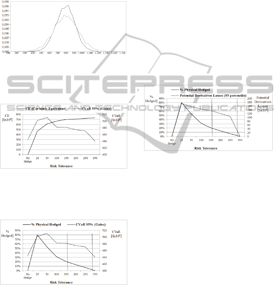
statistic. Figure 1 shows the high variability of Brent
prices returns, with other refined products exhibiting
a similar pattern.
Figure 1: Brent monthly price returns modelled with a
GARCH(1,1) model.
3.3 Correlation Modelling
Modelling correlation between the different products
prices, assuring nonlinear and complex
interdependencies, leads us to copula’s functions.
The Sklar (1959) theorem provides the theoretical
foundation for the application of copulas’ functions.
It assumes a stochastic multi-variable vector (X
1
,
X
2
,…X
n
), where X
i
is in our case the price of product
i with continuous marginals and cumulative density
ICORES2014-InternationalConferenceonOperationsResearchandEnterpriseSystems
130

function F
i
(x
i
)=P(X
i
≤ x
i
). Applying the probability
integral transform to each component:
[U
1
,U
2
,…U
n
]=[F
1
(X
1
),F
2
(X
2
),…,F
n
(X
n
)], having
U
i
є]0;1[ continuous margins.
The copula function C is defined as the joint
cumulative distribution function of [U
1
,U
2
,…U
n
],
where C[u
1
,u
2
,…,u
n
]=P[U
1
≤ u
1
,U
2
≤ u
2
,…, U
n
≤ u
n
].
The copula C contains all information on the
dependence structure between the components of
(X
1
, X
2
,…X
n
), whereas the marginal cumulative
distribution functions F
i
contain all information on
the marginal distributions. The great advantage of
copula’s functions is to allow the correlation pattern
modelled by the copula function to be independent
from the random variable X
i
marginal’s. Copula’s
functions are considered the most powerful and
flexible tool for portfolio management and risk
analysis (Jobst et al., 2006); (Rosenberg and
Schuermann, 2006); (Chollete, 2008).
3.4 Copula-GARCH Model
Natural Gas and Refining business units have very
narrow gross margins, which depend on complex
formulas involving several products prices,
demanding a powerful correlation method to assure
the margins’ values adhere to reality. Time series
functions and correlation functions, after long
testing, led us to the Copula-GARCH models (Lu et
al., 2011). Our method can be synthesized in three
steps: first, modelling the independent prices returns
with a GARCH model as described in (15) and,
second, find the best copula function to correlate
each GARCH price returns residuals z
t
.
z
t
r
t
t
(16)
Applying the SIC and the AIC criteria (Fermanian,
2005) we obtained the Student’s t copula (t-copula)
as the best copula function to model the prices return
residuals correlation. The Student’s t copula is
defined by:
Cu
1
;u
n
;
, d
T
d,
t
d
1
u
1
, t
d
1
u
n
(17)
where T is the t-copula with d degrees of freedom
and correlation matrix ρ, t
–1
is the inverse Student’s t
distribution with d degrees-of-freedom, and u
n
are
the marginal distributions of the n variables (the
price returns residuals, z
t
in our case).
The degree of tail dependency in the t-copula is
defined by d (degrees of freedom).
Finally, the third step evaluates each stochastic
price return p
t
using:
p
t
pe
r
t
(18)
where p is each forward price and r
t
is each price
return, given by the combination of a GARCH and a
t-copula function T being
Z
*
t
the residual correlated
with each other price returns residuals:
r
t
r
t1
2
t1
2
T
d,
t
d
1
u
t
Z
*
t
(19)
Unlike the Gaussian copula, the t-copulas have the
advantage of preserving the tail dependence in
extreme events (Asche et al., 2003), having steady
use in advanced portfolio risk estimation (Huang et
al., 2009), (Shams and Haghighi, 2013) and oil
hedging strategies (Chang et al., 2011).
4 RISK MODELLING
4.1 Risk Measures
Exposure, also called impact (Kaplan and Mikes,
2012), is the foreseen potential loss in money or in
other measurable variable if the risk occurs. The
importance of confronting an O&G gross margin
“exposure” with a measure of the respective
“uncertainty” is to guarantee that a company meets
its obligations with a previously imposed degree of
confidence (Haushalter, 2000). Artzner et al., (1999)
defined the axioms necessary and sufficient for a
risk measure to be coherent: positive homogeneity,
translation-invariance, monotonicity and sub-
additivity. Rockafellar and Uryasev (2000) proved
that standard deviation and Value-at-Risk (VaR)
created by J. P. Morgan (1992) are not coherent risk
measures, because the first violates translation
invariance and monotonicity, while VaR fails sub-
additivity. They proposed Conditional Value-at-Risk
(CVaR) as a coherent risk measure, which assures
the essential sub-additivity property and, as
presented in Figure 2 measures how large is the
average loss into the left tail ($720x10
6
), while VaR
only defines the loss frontier for a given probability
($600x10
6
).
Conditional Value-at-Risk (CVaR) is given by:
CVaR
1
EX
VaR
1
(20)
where X
α
is the value defined for having VaR for a
confidence level of 1 – α.
ManagingPriceRiskforanOilandGasCompany
131

Figure 2: Company downside earnings measured by VaR
and CVaR with a 95% confidence level.
4.2 Risk Tolerance
Utility theory, firstly proposed by Bernoulli (1738)
and developed by von Neumann and Morgenstern
(1944), allows determining a rational decision-
maker behaviour under risk and uncertainty. A
utility function u(x) describes a decision-maker
preferences and risk attitude allowing to translate,
e.g., dollars into utility units. A risk-averse decision-
maker would have a concave utility function,
meaning that she would exchange a higher expected
value of an uncertain game by a lower sure amount.
A risk-prone decision-maker (one that prefers a
higher expected value of an uncertain game to a
lower certain amount) would have a convex utility
function. A risk neutral decision-maker would have
a linear utility function.
The Certainty Equivalent (CE) is a key concept
in risk analysis. In the simple example lottery
depicted in Figure 3, the decision-maker may
consider the option “gamble”, with an outcome of
$100 (u(x) = 1) with a probability of 60%, and an
outcome of $0 (u(x) = 0) with a probability of 40%
indifferent to the option “not gamble”, if the certain
outcome of “not gamble” is $45. Thus, we would
say that CE = $45 and u($45) = u($100) × 0.6 +
u($0) × 0.4 = 0.6. The risk premium r (in $) is
given by:
r = E(x) – CE.
(21)
Consequently, for the above presented example, r =
($100 × 0.6 + $0 × 0.4) – $45 = $15.
Figure 3: Certainty equivalent meaning in a lottery.
Measuring corporate risk tolerance requires
assessing tradeoffs between potential upside gains
and downside losses under conditions of uncertainty.
As a result, the selection of the optimal
derivatives portfolio is influenced by the decision-
maker’s attitudes towards financial risk. This is the
point where utility theory commands the evaluation
of the optimal portfolio, assessing the decision
maker’s risk tolerance. The exponential utility
function (22) is one of the most widely used, and is
well tested on portfolio risk management in the oil
industry (Walls, 2005).
u(x) 1e
x
(22)
Its single parameter (the risk tolerance ρ), no initial
wealth dependence and constant absolute risk
aversion (–u''(x)/u'(x)=c
te
) (Pratt, 1964) explain the
exponential utility function wide use. In a lottery
game, the risk tolerance value ρ is the value that the
decision maker is willing to accept in order to play a
game where there are only two outcomes: winning
the amount ρ with a 50% probability or lose ρ/2 with
50% probability.
The exponential utility function performs better
than other utility functions, including the quadratic
utility function inherent to the Markowitz’s portfolio
optimization (Kirkwood, 2004) but using a utility
function advises a post sensitivity analysis to assure
the results robustness. The exponential utility
function certainty equivalent is:
CE
x
ln p
i
e
x
i
11
n
(23)
but can be simplified (Pratt, 1964, Clemen, 1996) for
outcomes with normal distributions (which is our
case, after K-S test) to:
CE
x
x
2
2
(24)
where μ(x) is the yearly average gross margin for the
company according to expression (13),
x
2
is the
gross margin variance and ρ is the company’s risk
tolerance.
4.3 Risk Tolerance Estimation
Numerous studies proposed evaluation methods for
corporate values of risk tolerance for exponential
utility functions. The most referred research suggests
setting the risk tolerance ρ at 6% of sales, 1 to 1.5
times net income, or 1/6 of equity in the “O&G”
companies (Howard, 1988). A more analytic
approach presented by Delquie (2008) proposes the
ICORES2014-InternationalConferenceonOperationsResearchandEnterpriseSystems
132

risk tolerance to be set to a fraction of the maximum
acceptable loss the company can afford for a given p
significance level, which can be considered a proxy
for the Value-at-Risk (VaR
1–p
):
VaR( p)
ln p
(25)
With a significance level p = 5% this implies that
the risk tolerance ρ is equal to one third of the
VaR
95%
.
Another common way to estimate corporate risk
tolerance is through a questionnaire answered by a
decision group panel who represents the company
risk profile (Board, CEO, CRO, CFO) for the most
important decisions.
Confronting each decision maker with a list of
questions in which he must choose between one of
two outcomes, x
1
or x
2
, with probabilities p
1
and p
2
,
respectively, it is possible to calculate iteratively the
certainty equivalent CE and the inherent risk
tolerance ρ that matches equation (23) (Walls
(2005)).
Another risk tolerance method estimation,
derived from the Capital Asset Pricing Method-
CAPM (Sharpe, 1964) is to assume the CE as the
effective cash-flow when each year t nominal cash-
flow CF
t
is discounted through the ratio of the risk
free rate r
f
to the rate that the company demands for
investments, the Weighted Average Cost of Capital
(WACC).
CE
t
CF
t
1r
f
t
1WACC
t
(26)
where CF
t
is the Project Cash-Flow in year t and r
f
is the free rate of return.
4.4 Risk Tolerance Results
Let us now explaining the results of the four
approaches employed:
a) With Howard’s we obtain the most conservative
estimation, e.g. one year of the company’s net
results is assumed to be the company’s risk
tolerance ($317x10
6
);
b) For Delquie’s, we estimate the VaR
95%
for the
company’s one year gross margin ($505×10
6
)
with p=5% in expression (25), which gives a risk
tolerance of $166
×10
6
;
c) For CAPM, we evaluated all the forecasted
project cash-flows 10 years ahead (essentially
E&P based) and we estimate the average
certainty equivalent applying (26), which gives a
risk tolerance of $220
×10
6
;
d) For the risk assessment questionnaire, we
confronted the CFO and his advisers with a set of
questions to evaluate the amount of money about
which they were indifferent, as a company, in
order to have a 50-50 chance of winning that
sum or losing half of it. A complementary set of
questions was made on the risk premium they
were willing to pay in order to receive with
certainty the average gross margin estimated for
next year’s budget. Applying expression (23) to
the first set of answers and expression (21) to the
second set of answers, it was possible to have a
series of risk tolerances values, with a mean of
$180
×10
6
and a standard deviation of $42×10
6
.
The risk tolerance results for the four methods are
presented in Table 1.
Table 1: Risk Tolerance results (in $10
6
).
Method Measure Value
Risk
Tolerance
Howard Net Income
317 317
Delquie VaR
95%
505 166
CAPM CE
370 220
Questionnaire Gross Margin
760
180
Delquie (2008) method has the most
conservative risk tolerance, while Howard’s method
estimated the highest value. The other ratios
proposed by Howard (equity and sales) give us even
larger risk tolerance values.
5 OPTIMIZATION RESULTS
In order to evaluate the consequences of the risk
tolerance estimates in Table 1, we ran optimizations
for a range of eight risk tolerance values, including
the four presented in Table 1, maximizing the
company certainty equivalent by inserting
expression (13) into expression (24):
max CE max m(d, m
e
, m
r
, m
g
)
m
2
2
(27)
We used a stochastic optimization algorithm
(Optquest, 2012) having the hedge quantities q
e
, q
s
,
q
c
and q
g
in expression (12) as the variables to be
determined. The stochastic price p
t
of each product
is embedded in the gross margin of each business
unit, m
e
, m
r
, m
g
and in the derivatives payout d, at
the same time.
After having achieved the optimal solution for
each of the eight risk tolerance values, we ran a
Monte Carlo simulation (5000 runs) using
ModelRisk (2012).
ManagingPriceRiskforanOilandGasCompany
133
The solutions from the integrated model (27)
have the advantage of obtaining the eight optimal
derivatives solutions while minimizing the “basis
risk” b. Figure 4 presents the density probability
curve for the un-hedged and hedged scenario for a
risk tolerance of $25
×10
6
.
Figure 4: Hedged and un-hedged margin for a $25×106
risk tolerance.
Figure 5 shows the risk tolerance impact in the
company certainty equivalent and into the CVaR
95%
(the risk measure).
Figure 5: CE and CVaR
95%
as a function of risk tolerance.
As risk tolerance increases, the certainty
equivalent increases, since the risk premium
decreases (see (24)). However, after a risk tolerance
of $ 50
×10
6
, we see a drop in the company CVaR.
Figure 6: CVaR
95%
and % Physical Hedged as a function
of Risk Tolerance ($10
6
).
Looking at Figure 6, the decrease in CVaR is
explained by the decreasing amount of derivatives d
in the optimized solutions, which allows greater
potential upside gains but greater potential downside
losses. The “% Physical Hedged” is the ratio
between the notional amounts of derivatives
contracts and the total physical company production,
both amounts in tons.
Less hedging means that the minimum gains (or
losses) get lower. Looking at the risk tolerance
vertical lines, the Delquie method implies about
20% hedging, the risk questionnaire about 15%,
CAPM about 7% hedging and Howard method
would imply only 3% hedging. The main question
that arises is about the “real” company risk
tolerance, because different risk tolerances imply
noticeable differences in terms of potential
derivatives losses, as is shown in Figure 7. Yearly
potential derivatives losses may vary from $20
×10
6
to $140×10
6
, which can have a heavy impact in the
Mark-to-Market (MTM) company quarterly
financial statements.
Figure 7: % Physical hedged and potential derivatives
losses as a function of risk tolerance.
6 MULTI-CRITERIA
EVALUATION
As we can observe in the results presented in section
5, the risk tolerance estimation widely affects the
hedging optimal solutions, and it is not clear if the
in-house risk assessment questionnaire defined
accurately the company risk profile. Therefore, we
will test in what extent the questionnaire reflects
with confidence the decision maker’s risk
preferences.
The company is interested in selecting the most
attractive hedging option from the set of eight
options previously built. However, the CFO and his
advisers, which constitute the company’s decision-
making group (DM), are not sure about which one to
select. In fact, they suspect that there is no option
that is the best according to all points of view that
came to their mind. To help the DM we developed a
multi-criteria evaluation model (Belton and Stewart
(2002)) using the MACBETH approach (Bana e
ICORES2014-InternationalConferenceonOperationsResearchandEnterpriseSystems
134

Costa and Vansnick, 1999; (Bana e Costa et al.,
2012), which required the group to: discuss their
points of view and select the criteria that should be
used to evaluate the hedging options; associate a
descriptor of performance to each criterion; build a
value function for each criterion; and weight the
criteria.
The additive value function model was selected
to provide an overall measure of the attractiveness of
each hedging option:
vx
1
,...x
n
w
i
v
i
x
i
i1
n
with
w
i
1,
i1
n
w
i
0
(28)
where v is the overall score of an hedging option x
with the performance profile (x
1
,…, x
n
) on the n
criteria, v
i
(i =1, …, n) are value functions, w
i
(i =1,
…, n) are the criteria weights. (Note that by applying
the additive value function model we are admitting
that a poor performance of an option in one criterion
may be compensated by good performances of that
option in other criteria. However, this working
hypothesis must be validated by the decision-making
group.)
The DM members discussed the points of view
they considered relevant for evaluating hedging
options having in mind the next year gross margin
budget as overall objective. After discussion, four
evaluation criteria were selected: 1) downside gains,
2) upside gains, 3) payout exposure and 4) risk
premium.
The performances of the hedging alternatives in
all criteria are their earnings expressed in $10
6
. The
5
th
and 95
th
earnings’ percentiles from the Monte
Carlo simulation results were used to define the
upper and lower reference levels, respectively, on
each descriptor of performance; three other
intermediate levels, between the upper and the lower
reference levels, were created on each descriptor of
performance. For example, Figure 8 presents the
performance levels of criterion “payout exposure”,
where 0 and 200 were defined as the upper and
lower reference levels, respectively, and 50, 100 and
150 are the intermediate levels; Figure 11 shows the
performance levels of all criteria).
Figure 8: Performance levels for the “payout exposure”
criterion (in $10
6
).
A value function was built for each criterion
using the MACBETH method and software
(www.m-macbeth.com), fixing 100 and 0 as the
value scores of the upper reference level and lower
reference level, respectively, on all criteria.
According to the MACBETH questioning protocol,
the decision-makers had to judge the difference in
attractiveness between each two levels of the
descriptor of performance using the semantic scale:
very weak, weak, moderate, strong, very strong or
extreme. For example, in the matrix of judgments for
criterion “payout exposure” (see Figure 9) the
decision-makers considered the difference in
attractiveness between $0 and $150
×10
6
to be very
strong (“v. strong” in Figure 9). After, M-
MACBETH proposed a value function scale
compatible with all the judgments inputted in the
matrix of judgements, using the linear programming
procedure presented by Bana e Costa et al. (2012).
The decision-makers were then asked to validate the
proposed scale in terms of the proportions between
the resulting scale intervals, and adjust them, if
needed. Figure 10 shows the value function scale for
the “payout exposure” criterion.
Figure 9: MACBETH matrix of judgments for the “payout
exposure” criterion.
Figure 10: Value function for the “payout exposure”
criterion (performances in $10
6
).
The following step consisted in eliciting weights
for the criteria. For that purpose five hedging
fictitious options were built: one option with a
performance at the upper reference level in one
criterion and performances at the lower reference
levels in the other three criteria with no repetitions
(what gives four fictitious options), and one
fictitious option with performances at the lower
reference levels in all the four criteria. Figure 11
ManagingPriceRiskforanOilandGasCompany
135
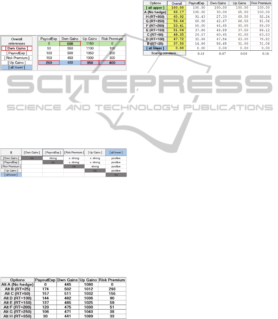
shows that the fictitious option “[Dwn Gains]” (see
the cell at top in column “Overall references” in
Figure 11) has a performance at the upper reference
level in criterion “Dwn Gains” (600) and
performances at the lower reference levels in the
other three criteria (“PayoutExp” – 200; “Up Gains”
– 950, “Risk premium” – 400). Then, the decision-
makers ranked the fictitious options by decreasing
order of their overall attractiveness, which resulted
in the rank shown in the “Overall references”
column in Figure 11.
Figure 11: Performance levels on the four criteria (in
$10
6
).
After, the decision-making group judged the
differences in attractiveness between each two
fictitious options, which allowed filling in the
MACBETH weighting judgments matrix show in
Figure 12. We underline that by accepting to make
these trade-offs, the group is validating our working
hypothesis of compensation between criteria.
Figure 12: MACBETH weighting judgments.
M-MACBETH then generated the criteria
weights by linear programming (see Bana e Costa et
al., 2012), which were show to the group for
validation and possible adjustment. The final criteria
weights (in %) were: Downside Gains (47%);
Payout exposure (33%); Risk premium (16%); and
Upside gains (4%).
In the last step, the performances of the eight
hedging options – from A (no hedge) until H
(tolerance risk of $350×10
6
) – were inputted in M-
MACBETH (see Figure 13).
Figure 13: Performances of the eight alternatives on the
four criteria (in $10
6
).
Note that the performances of the options are the
results generated for each of the eight risk tolerance
scenarios in section 5. With these data inputted the
partial (on each criterion) and overall value scores of
the hedging options were calculated by M-
MACBETH (see Figure 14).
Figure 14: Overall and partial value scores of the
alternatives and criteria weights.
In Figure 14 (column “Overall”) we see that the
most overall attractive option considering the
expressed preferences of the decision-makers is
option A (No hedge). Option H which corresponds
to the highest risk tolerance (ρ = $350
×10
6
), is
ranked second, whereas the least preferred hedging
option is B, which corresponds to lowest risk
tolerance (ρ = $25
×10
6
).
7 CONCLUSIONS
The multi-criteria evaluation of the hedging options
using the judgments of the same decision-makers
who answered the questionnaire gave us different
results in terms of preferred hedging options. The
most preferred hedging option “A”, and inherent
null hedging is closer to the Howard risk estimation
(ρ ≈ $350
×10
6
) and confirms Smith (2004)’s
findings that “large companies with reasonably
diversified shareholders should have risk tolerances
that are much larger than those typically suggested
in the decision analysis literature” (p. 114). In fact,
our research suggests the most preferred alternatives
have higher risk tolerance values than initially
estimated by the questionnaire.
With this research we show that it is possible to
perform a structured approach to model the entire
O&G company business model and evaluate price
risk management in an integrated way. Gross
margins from the three business units and a basket of
derivatives enter at once in a certainty equivalent
maximization problem and it becomes clear how the
hedging solutions vary with risk tolerance.
Defining a preliminary risk tolerance measure for
the company through a tailored risk assessment
ICORES2014-InternationalConferenceonOperationsResearchandEnterpriseSystems
136

questionnaire and comparing with other reference
methods of risk tolerance estimation allows
achieving preliminary solutions based on stochastic
portfolio optimization for each risk tolerance.
However, a multi-criteria final assessment should be
done, using the Monte Carlo simulation results, in
order to ascertain how decision-makers valuate the
underneath multiple consequences from each
hedging option. This multi-criteria final risk
tolerance evaluation can in fact help the company in
the always difficult decision “to hedge or not to
hedge” and, if yes, which amount to hedge.
It is important to note that these results were
obtained with data and preference judgements
concerning a specific moment in time. Few months
before or later, with different crude and refined
products prices, would lead to different decisions
under this approach. On the other side, each year,
the company has different goals, the market value
can grow or shrink along with the earnings and gross
margins. Further research should be done to evaluate
the results of the model in different price conditions
and involving other decision makers, preferably also
including board directors.
REFERENCES
Artzner, P., Delbaen, F., Eber, J.-M. & Heath, D. 1999.
Coherent measures of risk. Mathematical Finance, 9,
203–228.
Asche, F., Al, E., Gjølberg, O. & Völker, T. 2003. Price
relationships in the petroleum market: An analysis of
crude oil and refined product prices. Energy
Economics, 25, 289-301.
Bana e Costa, C. A., De Corte, J. M. & Vansnick, J. C.
2012. MACBETH. International Journal of
Information Technology & Decision Making, 11, 359-
387.
Bana e Costa, C. A. & Vansnick, J. C. 1999. The
MACBETH approach: Basic ideas, software, and an
application. In: Meskens, N. & Roubens M. R. (eds.)
Advances in Decision Analysis. Kluwer Academic
Publishers, Dordrecht, pp. 131-157
Belton, V. & Stewart, T. J. 2002. Multiple Criteria
Decision Analysis: An Integrated Approach, Kluwer
Academic Publishers, Boston, MA.
Bernoulli, D. 1738. Exposition of a new theory on the
measurement of risk. Econometrica, 22, 23-39.
Bollerslev, T. 1986. Generalized autoregressive
conditional heteroskedasticity. Journal of Economics,
31, 307-327.
Chang, C.-L., Mcaleer, M. & Tansuchat, R. 2011. Crude
oil hedging strategies using dynamic multivariate
GARCH. Energy Economics, 33, 912-923.
Chollete, L. 2008. Economic implications of copulas and
extremes. Penger og Kreditt - Norges Bank, 2, 56-58.
Clemen, R. T. 1996. Making Hard Decisions: An
Introduction to Decision Analysis. Duxbury Press,
Belmont, CA, 2nd edition.
Delquie, P. 2008. Interpretation of the risk tolerance
coefficient in terms of maximum acceptable loss.
Decision Analysis, 5, 5-9.
Energy Information Administration 2002. Derivatives and
risk management in the petroleum, natural gas, and
electricity industries. U.S. Department of Energy.
Fermanian, J.-D. 2005. Goodness-of-fit tests for copulas.
Journal of Multivariate Analysis, 95, 119-152.
Haushalter, D. 2000. Finance policy, basis risk and
corporate hedging: Evidence from oil and gas
producers. The Journal of Finance, 55, 107-152.
Howard, R. A. 1988. Decision analysis: Practice and
promise. Management Science, 34, 679-695.
Huang, J.-J., Lee, K.-J., Liang, H. & Lin, W.-F. 2009.
Estimating value at risk of portfolio by conditional
copula-GARCH method. Insurance: Mathematics and
Economics, 45, 315-324.
J.P.Morgan 1992. RiskMetricsTM—Technical Document.
In: J.P.Morgan/Reuters (ed.) Fourth Edition, 1996
Ji, Q. & Fan, Y. 2011. A dynamic hedging approach for
refineries in multiproduct oil markets. Energy, 36,
881-887.
Jin, Y. & Jorion, P. 2006. Firm value and hedging:
Evidence from U.S. oil and gas producers. The
Journal of Finance, 61, 893-919.
Jobst, N. J., Mitra, G. & Zenios, S. A. 2006. Integrating
market and credit risk: A simulation and optimisation
perspective. Journal of Banking & Finance, 30, 717-
742.
Kaplan, R. S. & Mikes, A. 2012. Managing risks: A new
framework. Harvard Business Review, 90, 48-60.
Kirkwood, C. W. 2004. Approximating risk aversion in
decision analysis applications. Decision Analysis, 1,
51-67.
Kretzschmar, G. L., Kirchner, A. & Reusch, H. 2008. Risk
and return in oilfield asset holdings. Energy
Economics, 30, 3141-3155.
Levy, H. & Markowitz, H. M. 1979. Approximating
expected utility by a function of mean and variance.
American Economic Review, 69, 308-17.
Lu, X. F., Lai, K. K. & Liang, L. 2011. Portfolio value-at-
risk estimation in energy futures markets with time-
varying copula-GARCH model. Annals of Operations
Research, doi: 10.1007/s10479-011-0900-9
Modelrisk 2012. Vose Software. http://
www.vosesoftware.com/
Nomikos, N. & Andriosopoulos, K. 2012. Modelling
energy spot prices: Empirical evidence from NYMEX.
Energy Economics, 34, 1153–1169.
Optquest 2012. OptTek Systems. http:// www.opttek.com/
OptQuest.
Platts 2012. Market Data – Oil, www.platts.com
Pratt, J. W. 1964. Risk aversion in the small and in the
large. Econometrica, 32, 122-136.
Quintino, A., Lourenço, J. C. & Catalão-Lopes, M. 2013.
An integrated risk management model for an oil and
gas company. Proceedings of EBA 2013, 16-19 July,
ManagingPriceRiskforanOilandGasCompany
137

Rhodes, Greece, pp. 144-151.
Reuters 2012. Commodities: Energy.
Rockafellar, R. T. & Uryasev, S. 2000. Optimization of
conditional value-at-risk. Journal of Risk, 2, 21-41.
Rosenberg, J. V. & Schuermann, T. 2006. A general
approach to integrated risk management with skewed,
fat-tailed risks. Journal of Financial Economics, 79,
569-614.
Shams, S. & Haghighi, F. K. 2013. A Copula-GARCH
Model of Conditional Dependencies. Journal of
Statistical and Econometric Methods, 2, 39-50.
Sharpe, W. F. 1964. Capital asset prices: A theory of
market equilibrium under conditions of risk. The
Journal of Finance, 19, 425-442.
Sklar, A. 1959. Fonctions de répartition à n dimensions et
leurs marges. Publications de l'Institut de Statistique
de l'Université de Paris, 229–231.
Smith, J. E. 2004. Risk sharing, fiduciary duty, and
corporate risk attitudes. Decision Analysis, 1, 114-127.
Von Neumann, J. & Morgenstern, O. 1944. Theory of
Games and Economic Behavior. Princeton University
Press, Princeton, NJ.
Walls, M. R. 2005. Measuring and utilizing corporate risk
tolerance to improve investment decision making. The
Engineering Economist, 50, 361-376.
ICORES2014-InternationalConferenceonOperationsResearchandEnterpriseSystems
138
