
Weighted SIFT Feature Learning with Hamming Distance
for Face Recognition
Guoyu Lu
1
, Yingjie Hu
2
and Chandra Kambhamettu
1
1
University of Delaware, Newark, U.S.A.
2
eBay Research, San Jose, U.S.A.
Keywords:
Face Recognition, SIFT Feature, Hamming Descriptor, Feature Transformation, Dimensional Reduction,
Feature Weighting.
Abstract:
Scale-invariant feature transform (SIFT) feature has been successfully utilized for face recognition for its
tolerance to the changes of image scaling, rotation and distortion. However, a big concern on the use of
original SIFT feature for face recognition is SIFT feature’s high dimensionality which leads to slow image
matching. Meanwhile, large memory capacity is required to store high dimensional SIFT features. Aiming to
find an efficient approach to solve these issues, we propose a new integrated method for face recognition in this
paper. The new method consists of two novel functional modules in which a projection function transforms
the original SIFT features into a low dimensional Hamming feature space while each bit of the Hamming
descriptor is ranked based on their discrimination power. Furthermore, a weighting function assigns different
weights to the correctly matched features based on their matching times. Our proposed face recognition
method has been applied on two benchmark facial image datasets: ORL and Yale datasets. The experimental
results have shown that the new method is able to produce good image recognition rate with much improved
computational speed.
1 INTRODUCTION
The basic task of face recognition is to identify the
query face image in the given images or videos, e.g.,
to compare a query face image with an image having
the already confirmed identification. Scale-invariant
feature transform (SIFT) (D.Lowe, 2004) is an algo-
rithm used in computer vision for translating images
into a set of features (SIFT features), each of which
is invariant to scaling and rotation, robust to distor-
tion and partially change in illumination. Owing to
the invariant characteristic, SIFT has been widely ap-
plied to the areas of object recognition, motion track-
ing, robot localization, to name but a few. How-
ever, some concerns have been raised about the effi-
ciency of SIFT feature even though it has the capabil-
ity of outperforming most conventional local feature
techniques for face recognition. One of the main is-
sues of using SIFT feature is the high dimensionality
of the feature which introduces heavy computational
cost for image matching. Pertaining to a real world
face recognition problem, usually a large number of
images are depicted by SIFT features in the train-
ing data, each being represented in a 128-dimensional
space. Such circumstance can significantly decrease
the image matching speed for face recognition. There
have been some attempts to use different approaches
to speed up the matching process, such as implement-
ing SIFT feature by multi-core systems (Zhang et al.,
2008) and building multi-scale local image structures
for face recognition (Geng and Jiang, 2011).
Inspired by LDAHash method (Strecha et al.,
2012), this paper proposes a new projection function
that reduces the curse of dimensionality and further
transforms the low dimensional feature space into a
Hamming space to reduce memory consumption and
improve matching speed. Meanwhile, we have de-
veloped a new method based on Hamming descrip-
tors utilizing the transitive closure of the descriptors
(Strecha et al., 2010) to improve image matching ac-
curacy. Unlike the method in which separated sub-
regions are represented by local binary pattern (LBP)
(Ahonen et al., 2006), our new Hamming descriptors
retain the scale invariant characteristic of SIFT and
allows the learning from the interesting points in the
training images. Thereafter, an improved grid-based
method (Bicego et al., 2006) uses the learned Ham-
ming descriptors to test the query image pertaining to
Lu G., Hu Y. and Kambhamettu C..
Weighted SIFT Feature Learning with Hamming Distance for Face Recognition.
DOI: 10.5220/0004859806910699
In Proceedings of the 9th International Conference on Computer Vision Theory and Applications (VISAPP-2014), pages 691-699
ISBN: 978-989-758-004-8
Copyright
c
2014 SCITEPRESS (Science and Technology Publications, Lda.)

a face recognition task.
SIFT feature is generally agreed to be capable
of producing satisfactory performance on affine and
scaling transformations (Kri
ˇ
zaj et al., 2010; Soyel and
Demirel, 2011). However, it lacks of the capability on
handling strong illumination changes and large rota-
tions, both of which may exist in face images, which
may produce a risk of relatively high false positive
matching rate in recognition. In the new proposed
method for face recognition, we use Random Sample
Consensus (RANSAC) (Fischler and Bolles, 1981)
to identify the correctly matched descriptors in the
learning period and then apply a weighting model to
assign higher weights to those more commonly cor-
rectly matched descriptors through an online recogni-
tion process. Thus the matching points retaining high
true positive rate will play a more essential role in the
matching process.
The remainder of the paper is organized as fol-
lows. Section 2 presents a review of the related work
in which SIFT feature has been used for face recogni-
tion. Section 3 proposes our new method that projects
SIFT descriptors into a lower dimension Hamming
space. Section 4 describes a new weighting method
for improving matching accuracy. Section 5 presents
the experimental results and the findings, followed by
the conclusion of this paper in section 6.
2 RELATED WORK
During the last two decades, significant progress has
been made in face recognition with the development
of a variety of methods. Classical statistical algo-
rithms have been widely used for face recognition
problems and have performed well under some cir-
cumstances. Eigenfaces (Turk and Pentland, 1991)
and Fisherfaces (Belhumeur et al., 1997; Jiang, 2011)
are two classical face recognition methods that em-
ploy principal component analysis (PCA) and lin-
ear discriminant analysis (LDA), respectively. Eigen-
faces and Fisherfaces based methods handle face im-
ages as a global feature, which is sensitive to face ex-
pression and head rotation. Thus, the performance
from Eigenfaces and Fisherfaces based methods is not
promising when face images have certain changes or
distortions.
To mitigate the various issue raised by global fea-
ture method in face recognition applications, local
features have been deployed for their invariant char-
acteristics on face scaling, rotation and other changes.
Recent research attempts to use local feature for face
recognition. SIFT feature is a method that is invari-
ant to image scale and rotation, which offers a ro-
bust matching technique to achieve high face recog-
nition rate with only a small set of features trans-
lated from face images. It has been incorporated into
a variety of computational models and systems for
image recognition problems, including face recogni-
tion. One representative work can be found in (Bicego
et al., 2006). They applied SIFT features to a grid-
based method for image matching in which the aver-
age minimum pair distance was used as the match-
ing criterion. Their approach not only decreased the
false positive rate (FPR) of the image matching, but
also reduced the computational complexity. To pro-
duce high recognition rate, SIFT feature was em-
ployed for describing local marks (Fernandez and Vi-
cente, 2008; Rosenberger and Brun, 2008) and was
combined with a clustering-based method (Luo et al.,
2007). In the clustering-based method, face images
are usually clustered into 5 regions: two eyes, nose,
and mouth corners. Although the recognition accu-
racy rate can be slightly improved compared with the
method in (Bicego et al., 2006), extra computational
time for clustering is required.
Recently, more sophisticated face recognition
methods using SIFT feature have been developed and
applied to real world applications. Geng and Jiang
(Geng and Jiang, 2011) introduced a method that
created a framework trained by multi-scale descrip-
tors on the smooth parts of face. To reduce the fea-
ture quantization error, SIFT feature has been incor-
porated with a kernel based model for face recog-
nition, such as Sparse Representation Spatial Pyra-
mid Matching (KSRSPM) method (Gao et al., 2010).
Also, SIFT feature has been studied for solving 3D
face recognition problems and reported to able to pro-
duce high recognition accuracy (Mian et al., 2008).
Our method utilizes the grid-based approach for
local feature matching with the adjustment of mak-
ing the method more robust on face rotation. For lo-
cal feature matching, we reduce the dimensionality
of the original SIFT feature by our learned projection
matrix. Furthermore, the learned low dimensional lo-
cal feature is mapped to Hamming space. Each bit of
the learned Hamming descriptor is weighted by our
ranking method to reduce the ambiguity in matching
the descriptors. We also give the weight for each de-
scriptor to highlight the most discriminant descriptor,
which improves the face recognition accuracy.
Grid-based methods offers an effective and scal-
able approach for building high performance system
to solve face recognition problems (Bicego et al.,
2006; Luo et al., 2007; Majumdar and Ward, 2009).
The basic idea behind grid-based methods is to di-
vide a face image into several subregions to reduce
image matching time and false positive rate. Com-
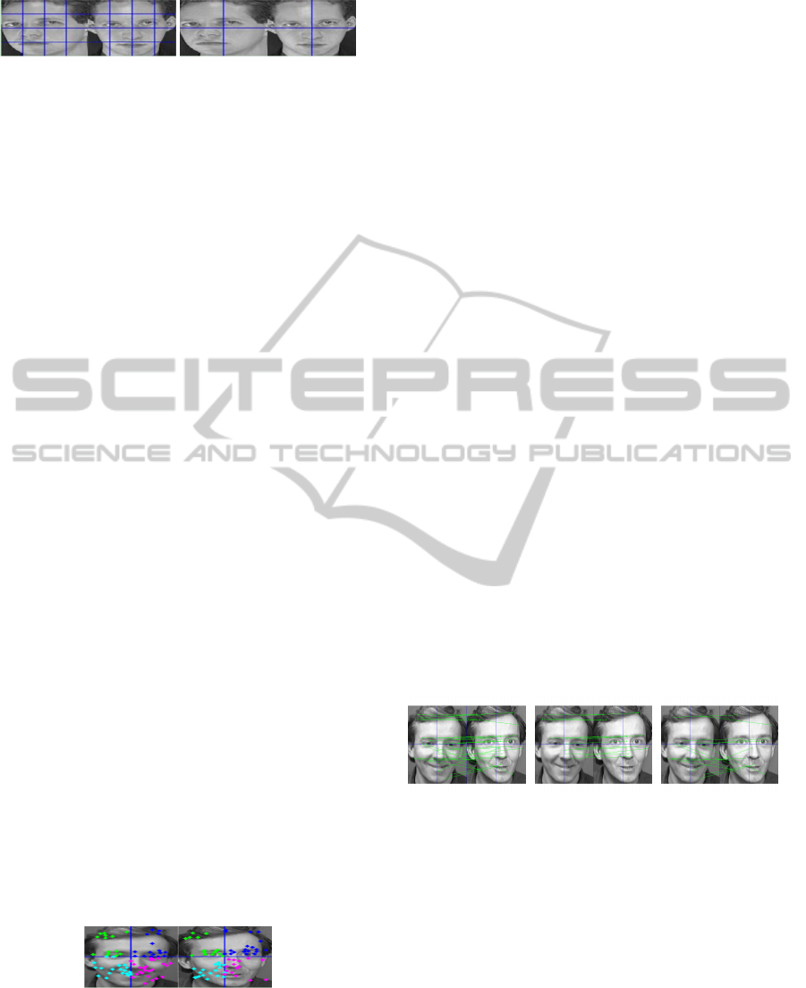
(a) Face images are di-
vided into 4 ∗ 4 grids,
where the left eyes and
left mouth corners are not
in the same corresponding
grid
(b) Face images are di-
vided into 2 ∗2 grids. The
eyes and mouth corners ba-
sically locate in the same
grids, e.g., the left eyes and
left mouth corners are in
the same grid, respectively.
Figure 1: An example of face images divided into different
number of sub regions.
pared with cluster-based image matching methods,
grid-based methods are able to produce high recog-
nition rate, but with much less computational time.
Such characteristic makes this approach an appropri-
ate method for handling large face image databases.
A grid-based method needs to specify an appropri-
ate number of subregions to divide face images. For
example, to improve the computing speed, 4 ∗4 grids
(16 subregions) are specified in (Majumdar and Ward,
2009) for facial image matching. However, too many
subregions may decrease rotation invariance and in-
crease the matching error rate within the correspond-
ing subregions. Figure 1 gives a simple example to
demonstrate the difference of face image division us-
ing different number of subregions for face image di-
vision. As shown in Figure 1(a), 4 ∗4 grids are used
to divide face images. The same components of a per-
son’s face images are not in the same corresponding
grids, e.g. the left eyes in Figure 1(a) are not in the
same gird (grid(2,1)). Using 2 ∗ 2 grids in Figure
1(b), the same components (the left eyes) in the two
face images are in the same grid (grid(1,1)). There
is no significant difference between using 2 ∗2 grids
and 4 ∗4 grids in terms of matching speed, as the
features are unequally extracted from subregions (i.e.
most features are extracted from certain key parts in a
face, such as eyes and mouth corners). Figure 2 gives
an example of extracting features from two facial im-
ages using a grid-based method. Due to the efficiency
in fast matching computing and rotation invariance,
we choose 2 ∗2 grids for dividing the symmetric parts
of face images in our proposed method.
Figure 2: The features extracted from two images. Most
features are extracted from the key parts of faces, such as
eyes, eyebrows, nose and mouth.
3 DESCRIPTOR LEARNING
3.1 Real-value Descriptor Learning
LDAHash (Strecha et al., 2012) is an approach that
projects the original high dimensional local features
into lower dimensional binary feature space. The ap-
proach generates compact binary vectors transformed
from original real-value vectors and preserves the
properties of the original vectors extracted from fa-
cial images. Using binary descriptors, LDAHash re-
quires much less memory storage than real-value de-
scriptors and leads to faster similarity computation for
image retrieval. Additionally, LDAHash enlarges the
distribution distance between positive and negative
pairs by a projection function, where negative pairs
are randomly selected. Nevertheless, in real world im-
age recognition problems, the similarity between pos-
itive and random negative descriptor pairs can be very
small. Thus, one of the main challenges in face recog-
nition research is how to use the local matching fea-
tures (e.g. SIFT features) to distinguish the positive
descriptors from negative descriptors. In many cases,
there are some features (descriptors) that are very
close to the query features (descriptors). Such fea-
tures are defined as nearest neighbor negative descrip-
tors (Philbin et al., 2010), if they are not explained by
the RANSAC transformation. The matching features
are considered to be the positive descriptors pairs if
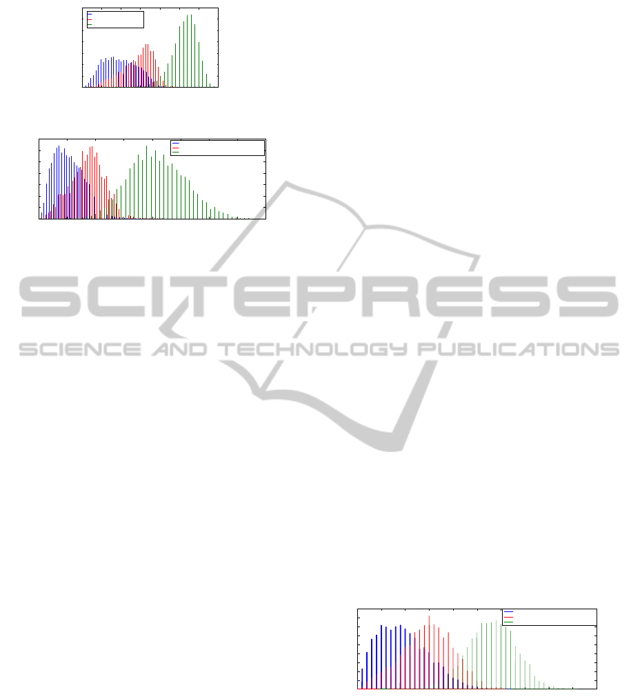
they satisfy the RANSAC transformation. Figure 3
gives an example that demonstrates the difference be-
tween the positive descriptors and the nearest neigh-
bor negative descriptors for facial image matching.
(a) The initial
matching out-
come obtained
by a Grid-based
matching method.
(b) The positive
descriptor pairs
are fitted in the
RANSAC trans-
formation for
image matching.
(c) The near-
est neighbor
negative descrip-
tors created by
SIFT algorithm
which are not
satisfied with
the RANSAC
transformation.
Figure 3: An example of positive and the nearest neighbor
negative descriptors for face recognition.
Differences of covariance (DIF) was used in LDA-
Hash for distinguishing positive and negative descrip-
tors to controll their weights (Strecha et al., 2010).
The performance obtained by DIF is heavily depen-
dent on the appropriate choice of the relevant param-
eters used for assigning weights, while other settings

may result in the failure of eigen-decomposition for
real-value scope. Such issue poses a big challenge to
LDAHash based face recognition methods.
To deal with the issues of reducing feature di-
mensionality and finding the appropriate parameters
for LDAHash method, we propose a new projecting
function that takes into account the nearest neighbor
negative pairs for similarity matching. This new de-
veloped projecting function is used for reducing the
curse of feature’s dimensionality and separating pos-
itive, nearest neighbor negative and random negative
pairs as well. Although most mismatching is caused
by the nearest neighbor negative pairs, random nega-
tive pairs should not be neglected as they may crowd
into the group of the nearest neighbor negative pairs
after the projection.
A loss function is used in the proposed projection
function to reduce the mismatching between positive
and negative descriptor pairs:
L =αM ·{P ·(X
T
p
Y
0
p
) ·P
T
|P}
−βM ·{P ·(X
T
NN
Y
0
NN
) ·P
T
|NN}
−γM ·{P ·(X
T
RN
Y
0
RN
) ·P
T
|RN}
(1)
where:
X,Y
0
are two descriptors’ matrices;
P, NN and RN represent the positive pairs, near-
est neighbor negative pairs and random negative
pairs, respectively;
α,β,γ are the three weight variables for positive,
nearest neighbor negative and random negative
pairs, respectively;
T represents transformation matrix;
M is a function for calculating the average dis-
tance;
P is a projection function.
In our experiment, the three groups of descriptor
pairs (P, NN, RN) initially have the equal weights, i.e.
α, β and γ have the same initial value.
Here, we substitute M{X
T
Y
0
|·} with a covariance
matrix denoted by
∑
, and rewrite Eq.1 as:
L =αM(P
∑
P
P
T
) −βM(P
∑
NN
P
T
)
−γM(P
∑
RN
P
T
)
(2)
Then, we can have the following equations
derived from Eq.2:
L =αM(P
∑
P
P
T
)
−{βM(P
∑
NN
P
T
) + γM (P
∑
RN
)P
T
)}
(3)
L =αM(P
∑
P
P
T
)
−M{P (β
∑
NN
+ γ
∑
RN
)P
T
}
(4)
L = αM(P
∑
P
P
T
) −M (P
∑
SN
P
T
) (5)
where,
∑
SN
= β
∑
NN
+ γ
∑
RN
(6)
The coordinates are transformed by pre-
multiplying
∑
SN
(−1/2)
and
∑
SN
(−T /2)
, so that
the second term of Eq. 6 turns into a constant that the
loss function
e
L does not need to take into account.
e
L ∝ M{P
∑
SN
(−1/2)
∑
P
∑
SN
(−T /2)
P
T
}
= M{P
∑
P
∑
SN
(−1)
P
T
}
(7)
Eigen-decomposition can be used here for cal-
culating the loss function, since
∑
P
,
∑
SN
(−1)
and
∑
P
∑
SN
(−1)
are symmetric positive semi-definite ma-
trices. The projection function minimizes the loss
function and yields the k smallest eigenvectors of
∑
P
∑
SN
(−1)
. The weights are given to the three classes
of descriptor pairs (α, β and γ) for optimizing the pro-
jection function.
The main difference between our proposed
method and DIF method in LDAHash is that the
choice of parameters does not create a non symmetric
positive semi-definite matrix, i.e. our proposed pro-
jection is able to produce more reliable results for di-
mension reduction. With our new projection function,
the values of α, β and γ are not critical to the perfor-
mance of the given image matching task, while the ra-
tio of β and γ plays an important role in the projection
function. Using the new projection function, the sce-
nario of setting the extreme values of β or γ will be the
same as ignoring random negative or nearest neighbor
negative pairs. Under such scenario, the projected de-
scriptors will still be better classified than those in the
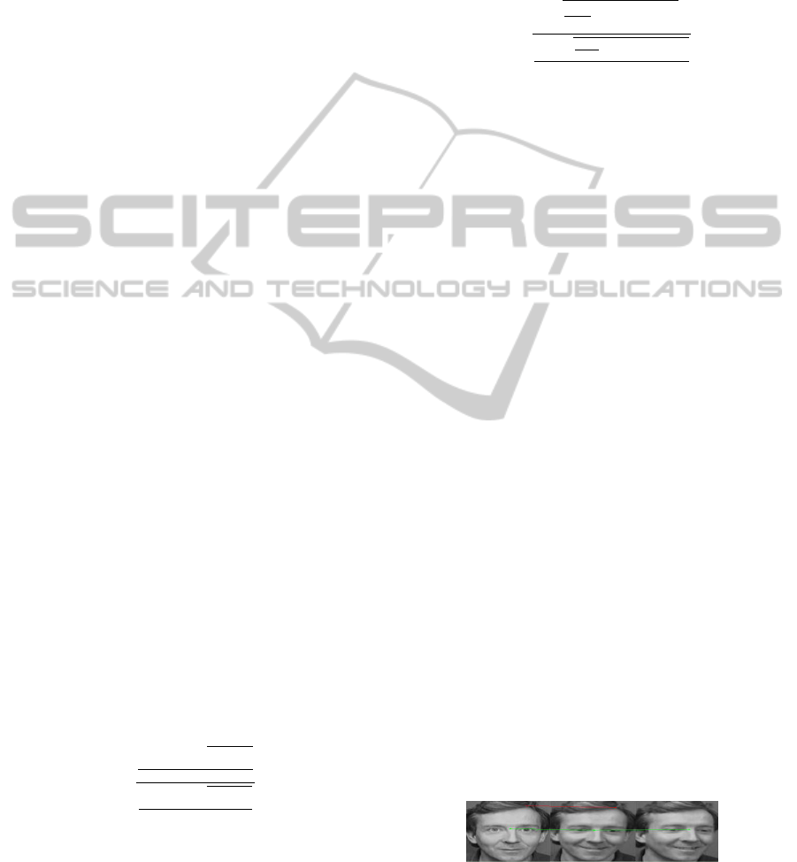
original feature space. The results of the three classes
of descriptor pairs before and after the projection are
plotted in Figure 4. The descriptor pairs are projected
into a 64-dimensional space.
As shown in Figure 4, the distribution of positive
descriptor pairs becomes much more compact after
the projection than before the projection, compared
to the nearest neighbor negative and random negative
pairs. Also, random negative descriptor pairs are dis-
tributed in a more sparse manner. More importantly,
the distribution distance between positive descriptors
and the nearest neighbor negative descriptors is en-
larged, which is the same for positive descriptors and
random negative descriptors. Meanwhile, the over-
lapping area between positive pairs and the nearest
neighbor negative pairs is shrunken. Such phenom-
ena suggest that the improved performance of image
matching can be certainly guaranteed using the pro-
jected real-value features in a low-dimensional space.
0 100 200 300 400 500 600 700
0
0.02
0.04
0.06
0.08
0.1
0.12
0.14
Pair distance
Percentage
Original descriptor pair distance
Positive pair distance
Nearest neighbor negative pair distance
Random negative pair distance
(a) The original pair distance be-
fore the projection.
0 500 1000 1500 2000 2500 3000 3500 4000
0
0.01
0.02
0.03
0.04
0.05
0.06
0.07
Pair distance
Percentage
Pair distance after projecting into 64−D space
Positive pair distance
Nearest neighbor negative pair distance
Random negative pair distance
(b) The new pair distance after the projection.
Figure 4: Descriptor pairs’ distance histogram before and
after they are projected into a new space, where X-axis is the
distance of the descriptor pairs while Y-axis represents the
percentage. (Blue, red and green are separately represent-
ing positive, nearest neighbor negative and random negative
descriptor pairs.)
3.2 Hamming Descriptor Projection
To reduce the computational cost, our proposed new
method further projects the new low dimensional de-
scriptors into a Hamming space. As discussed in
the previous sections, the computation using Ham-
ming vectors is much faster than that using real-value
vectors. Moreover, the memory required for storing
descriptors can be significantly reduced if real-value
descriptors are transformed into a Hamming space.
Hereby, the projection from a real-value space to a
Hamming space is formulated as:
y = I
A
(x −θ) (8)
where x is the projected real-value descriptors, y
is the descriptors in a Hamming space and θ is a
threshold to be learned to ensure that the projected
Hamming descriptors best represent the original real-
value descriptors’ property; I
A
denotes a sign indica-
tor function.
In our proposed projection function, we introduce
a set of nearest neighbor negative descriptors to opti-
mize a threshold θ and give the weights to different
false matching rates based on three categories of de-
scriptors calculated by LDAHash method. The basic
idea here used for optimizing θ is to either minimize
the false matching rate or maximize the true match-
ing rate. In this study, we choose minimizing the false
matching rate to optimize θ. The false negative (FN)
rate can be computed using the following equation:
FN(θ) =Pr{min(x
P
,y
P
) < θ ≤ max(x
P
,y
P
)|P}
=Pr{(min(x
P
,y
P
< θ)|P}+ 1
−Pr{(max(x
P
,y
P
) < θ)|P}
=cd f {min(x
P
,y
P
)|P}−cd f {max(x
P
,y
P
)|P}
(9)
cd f is the cumulative distribution function. The
false positive rate is divided into two parts: one is
used for describing the nearest neighbor negative de-
scriptors and is denoted by FPN; the other part is
for random negative descriptors and is denoted by
FPR. FPN and FPR can be computed by the follow-
ing Eq.10 and Eq. 11:
FPN(θ) =Pr{min(x
NN
,y
NN
) ≥ θ
∪max(x
NN
,y
NN
) < θ)|NN}
=1 −cd f (min(x
NN
,y
NN
)|NN)
+ cd f (max(x
NN
,y
NN
)|NN)
(10)
FPR(θ) =Pr{min(x
RN
,y
RN
) ≥ θ
∪max(x
RN
,y
RN
) < θ)|RN}
=1 −cd f (min(x
RN
,y
RN
)|RN)
+ cd f (max(x
RN
,y
RN
)|RN)
(11)
The overall false matching rate is given by:
F(θ) = α
0
FN + β
0
FPN + γ
0
FPR (12)
α
0
, β
0
and γ
0
are the weights given to the different
false rates. The higher the α
0
, the lower the false neg-
ative rate is. cd f is a cumulative distribution function
that creates the distribution corresponding to every θ
to be tested. In our experiment, α
0
, β
0
and γ
0
are ini-
tialized to be 1 and θ is accurate to one decimal place.
The distance between three classes of descriptor pairs
is shown in Figure 5.
0 5 10 15 20 25 30 35 40 45 50
0
0.01
0.02
0.03
0.04
0.05
0.06
0.07
0.08
0.09
Hamming descriptor pair distance
Percentage
Pair distance after projecting into 64−D Hamming space
Positive pair distance
Nearest neighbor negative pair distance
Random negative pair distance
Figure 5: The descriptor pair distance after projecting into a
Hamming space. (Blue, red and green are separately repre-
senting positive, nearest neighbor negative and random neg-
ative descriptor pairs.)
From Figure 5, we can see that the descriptors in
a low-dimensional Hamming space performs more or
less the same as the transformed SIFT descriptors in a
64-dimensional (64-D) space. The binary descriptor
preserves the properties of 64-D descriptors and per-
forms much better than using 128-D SIFT features.
3.3 Bit Ranking in Hamming Space
Hamming descriptor is advantageous for its efficient
storage and easy computation. However, as Hamming
descriptors have only two value options for each di-
mension and the length of the descriptor is limited,
there usually exist multiple descriptors sharing the
same Hamming distance to the query descriptor. In
dealing with this problem, we rank each bit of the
Hamming descriptor and give different weights for
the dimensions, which will help to reduce the ambi-
guity in matching the descriptors.
Ideally, in Hamming space, if two descriptors
are coming from the same point(positive descriptors),
they should share the same value in the corresponding
dimension. However, in practice, there will be several
bits differ for the two descriptors from the same pos-
itive descriptor pair. The value of each dimension of
the descriptor is distributed differently. This results in
the difference of the discrimination power among all
the descriptors’ dimensions. For example, two Ham-
ming descriptors H1 and H2 have the same distance
to the query descriptor Hq. H1 differs from Hq in
the ith bit, while H2 differs from Hq in the jth bit. If
ith dimension has more discrimination power than the
jth dimension, we consider the distance between H1
and Hq is larger than the distance between H2 and
Hq. We learn the discrimination power by complying
with the idea of decreasing the positive descriptors’
distance and increasing the negative descriptors’ dis-
tance.
As descriptors will loose information after hash-
ing, we use the real-value projected descriptors to
learn the ranking. If the descriptors’ value of the
same point is quite similar and very distant to the de-
scriptors’ value of other points, the hashing results
of this point’s descriptors have strong confidence to
be correct. On the other side, if the same points’
descriptors’ value is not distinguishable from other
points, the Hamming descriptor of this dimension is
less credible than other dimensions with high correct-
ness confidence. For the ith dimension, we calculate
the weight as the following equation:
W
i
=
∑
(y
i
,y
0
i
)∈N
√
(y
i
−y
0
i
)
2
Nbn
∑
(x
i
,x
0
i
)∈P
√
(x
i
−x
0
i
)
2
Nbp
(13)
Where Nbn and Nbp are representing negative and
positive descriptor pairs number. For all the nega-
tive descriptor pairs (e.g.(y
i
,y
0
i
) ∈N), we calculate the
sum of all the descriptor pairs’ Euclidean distance and
further divide the sum by the negative descriptor pairs
number. The same for positive descriptors. The di-
vision result will be the weight for this dimension.
However, the complexity of computing the distance of
positive and negative descriptor pairs is O(n
2
), which
consumes a large amount of time. As an alternative,
we use the positive descriptor pairs’ standard devia-
tion to substitute the Euclidean distance, as Eq.14.
W
i
=
q
1
N−1
∑
N
1
(y
i
−µ)
2
∑
N p
1
q
1
NDes
∑
NDes
1
(x
i
−µ
des
)
N p
(14)
In Eq.14, N is the number of all the descriptors
and µ is the mean of all the descriptors’ ith dimen-
sion value. For the positive standard deviation part,
N p is the number of different points. Ndes repre-
sents the descriptor number of the current point. µ
des
is the ith dimension’s mean value of the descriptors
from the same point. Both Eq.13 and Eq. 14 can
describe the distribution of the descriptor’s value be-
fore hashing. The larger negative descriptor value dis-
tance and the smaller positive descriptor value dis-
tance, the more confidence we have for this dimen-
sion. As a result, we will give a higher weight to this
dimension. As Eq.14 uses standard deviation to sub-
stitute the Euclidean distance of each descriptor pair,
the time complexity is O(n), which is much smaller
than the method used in Eq. 13.
4 FEATURE WEIGHTING
A weighting function with a RANSAC model is used
for identifying the true positive matching between the
descriptors in two images. Generally, the correctly
matched points during the training stage are more
likely to contribute better performance for the testing
data. Therefore, different weights are assigned to the
different points, based on their matching performance
obtained in the training stage.
Initially, we give all the points the weight of 1.
The weights of the points will increase by 1, if the
descriptors extracted from the points satisfying the
RANSAC transformation during the image matching.
Figure 6 gives such an example.
Figure 6: The points that fit RANSAC transformation in
three images. The green point in the middle image matches
the corresponding points in the left and right images, while
the red point in the middle image only matches the corre-
sponding points in the left image.
In Figure 6, the weight of the green point in
the middle image will be increased to 3, since it is
matched to the corresponding points in the left and
right images. The red point in the middle image
only matches the corresponding point in left image,
so that its weight will be increased to 2. The larger
the weight, the more important the features for face
recognition. Our main goal here is to highlight the
true positive matching points. RANSAC may mis-
takenly identify the correct matching points as false
matching points, when there are some rotation and il-
lumination changes in the matching images. For this
reason, we do not give any penalty to the false positive
matching points, and the matched point (true posi-
tive matching point) should be weighted n times more
than an unmatched (false positive) point. Here n rep-
resents the number of matching between query and
training images. For example, let us consider a test
using the same images from Figure 6. The feature
highlighted in green (with weight ’3’) have the more
importance than the feature in red (with the weight
’1’) in terms of improving face recognition rate.
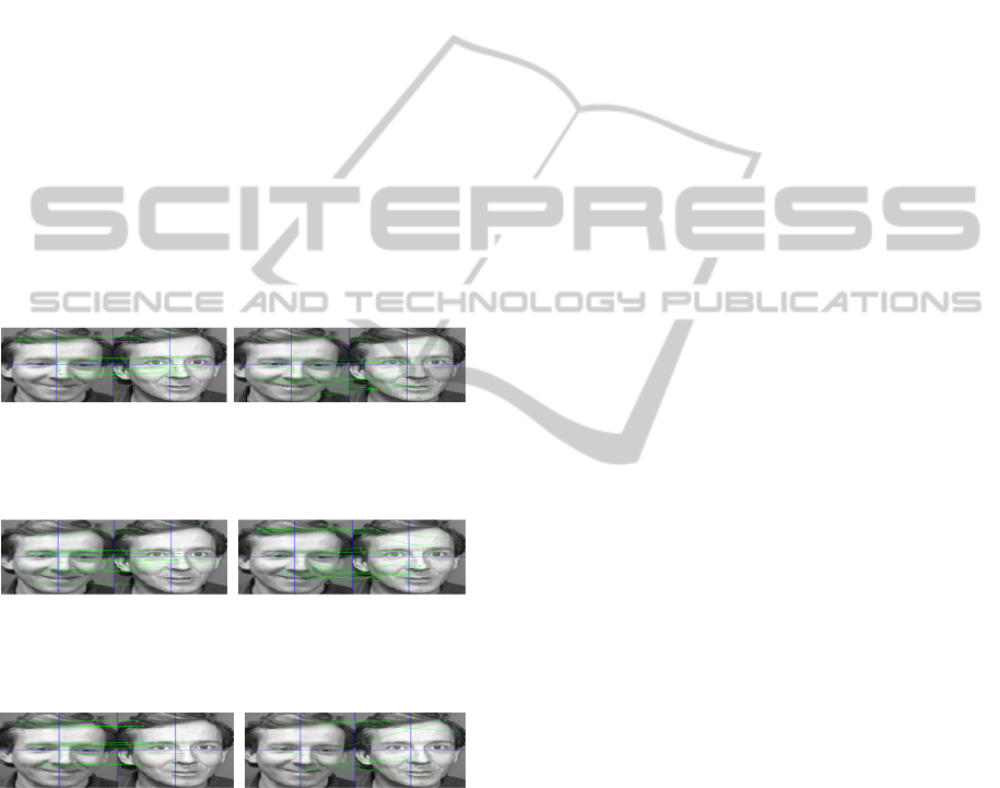
(a) The face image matching result obtained by using the
original 128-D SIFT features. It consists of 16 true positive
matching (including 3 RANSAC misjudges) and 11 false
positive matching (excluding RANSAC misjudges). The
true positive matching rate is 59.2%.
(b) The face image matching result obtained by using the
64-D projected real-value features. It consists of 20 true
positive matching (including 6 RANSAC misjudges) and 12
false positive matching (excluding RANSAC misjudges).
The true positive matching rate is 62.5%.
(c) The face image matching result obtained by using the
the 64-D projected Hamming descriptors. It consists of 13
true positive matching (including 2 RANSAC misjudges)
and 6 false positive matching (excluding RANSAC mis-
judges). The true positive matching rate is 68.4%.
Figure 7: The comparison of the face image matching per-
formance obtained using three feature techniques.
The whole learning process is complex but can be
performed offline. During the offline learning step, all
the image features can be projected into a Hamming
space and stored into a binary file, which requires
much smaller memory capacity. After the recognition
methods have been trained through an offline step, the
online face recognition process for testing will be per-
formed much faster using Hamming descriptors.
5 EXPERIMENT AND
DISCUSSION
5.1 Dataset
Two benchmark face image datasets (ORL and Yale
dataset) are used in this study for evaluating our pro-
posed for face recognition. The first dataset is ORL
dataset (Samaria and Harter, 1994) that contains the
subjects (face images) collected by AT&T Laborato-
ries and Cambridge University Engineering Depart-
ment. The dataset consists of ten different individ-
uals, each having 40 distinct subjects. The images
were taken at different time moments with different
lighting conditions. Thus, the face images in the
dataset were with the variation affected by different
factors, such as facial expressions (e.g. open/closed
eyes, smiling/not smiling) or facial details (with
glasses/without glasses). The second dataset is the
Yale face database (Belhumeur et al., 1997) that con-
tains 165 grayscale images in GIF format collected
from 15 individual participants. Each individual has
11 images under different viewing conditions with
various facial expression or configuration, such as
the illumination (left or right light), with or without
glasses, and the emotions (happy, sad, surprised, etc).
Both of ORL and Yale datasets are publicly available.
5.2 Experiment Results
To evaluate the performance of our new proposed
method for face recognition, we present a compara-
tive experiment using the new learned 64-D projected
Hamming descriptors, the projected 64-D real-value
descriptors and the original 128-D SIFT features. Fig-
ure 7 illustrates the comparison of matching results.
The experimental result shows that the matching
accuracy from the new learned Hamming descriptors
is better than that from the original SIFT features.
More importantly, Hamming descriptors reduces the
false positive rate compared with using the original
SIFT features.
Additionally, to test the robustness of our new de-
veloped method, we further applied it on the stan-
dard ORL face database (head rotation) and Yale face
database (illumination change). We use half images
for training and the rest for testing. Compared to
classical PCA (Turk and Pentland, 1991), LDA (Bel-
humeur et al., 1997), conventional SIFT method (Ma-
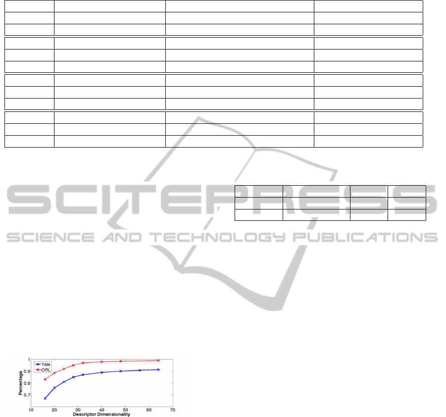
Table 1: Testing accuracy of ORL and Yale data using different face recognition methods.
Database PS-64 HS-64 HS-32
Yale 92.9% 91.8% 87.3%
ORL 99.1% 99.1% 97.3%
Database HS-16 PCA LDA
Yale 67.8% 67.8% 82.4%
ORL 83.3% 88.6% 91.2%
DataBase SIFT Method (Wright and Hua, 2009) Method (Lu et al., 2010)
Yale 85.8% 91.4% 89.1%
ORL 95.8% 96.5% 94.8%
DataBase Method (Liu et al., 2012) Method (Yang and Kecman, 2010) -
Yale 83.4% - -
ORL 98.9% 98.4% -
jumdar and Ward, 2009) and some state-of-art meth-
ods ((Wright and Hua, 2009; Lu et al., 2010; Liu
et al., 2012; Yang and Kecman, 2010)), Table 1 sum-
marizes the experimental results for face recognition.
We denote the projected 64-D real-value descriptors
as PS-64 and the 64-D Hamming descriptors as HS-
64, and summarize the testing accuracy in Table 1.
The experimental results clearly show that the
proposed face recognition methods using low-
dimensional features (either real-value or binary)
have consistently produced good matching accuracy
on both ORL and Yale data. In this study, we have
also investigated the dependency of face recognition
accuracy on the different number of Hamming de-
scriptor dimension and plotted the results in Figure
8.
Figure 8: Accuracy and Hamming descriptor dimensional-
ity diagram on ORL and Yale data. Both are tested from 16
dimensions to 64 dimensions.
In general, the higher the Hamming descriptor di-
mension used, the better the matching accuracy. The
accuracy increases sharply from 16 dimension to 32
dimension. After 32 dimension, the accuracy in-
creases smoothly.
As the similarity computation of Hamming de-
scriptors is based on bit operation, the time for cal-
culating distance between extracted descriptors is
largely reduced. Table 2 gives the average time per-
formance on computing descriptors’ distance of each
image pair based on SIFT descriptors and our learned
Hamming descriptors.
From Table 2, we can see that our Hamming de-
Table 2: Average time consumption on computing descrip-
tors’ distance of each image pair.
Database Origianl SIFT HS-64 HS-32
Yale 0.62s 0.25s 0.22s
ORL 0.075s 0.028s 0.020s
scriptor largely reduce the time on computing descrip-
tor distance. The 32 dimensional Hamming descrip-
tor achieves almost 3 times accelaration on similarity
computation compared with SIFT descriptor based on
grid method, while increasing the accuracy.
6 CONCLUSIONS
It is always challenging to improve the matching ac-
curacy and reduce the computational cost simulta-
neously in face recognition applications. In the in-
troduction section, we have described the motivation
of using the projected Hamming descriptors for face
recognition. For this purpose of dealing with such
issue, we have developed a novel method for face
recognition problems which uses a new projection
function combined with a weighting function to re-
duce the high dimensionality of SIFT features.
Our proposed method offers a good solution to
handle the large datasets with enormous features,
owning to its ability of fast computing and small
memory requirement. In this study, the new face
recognition method were fulfilled in two ways: (1)
using a projection function to transform original SIFT
features into a low dimensional space, and (2) using
a more sophisticated projecting function for generat-
ing Hamming descriptors which reduces the memory
requirement and improves the computational speed.
To optimize the descriptors, we introduced a new fea-
tures weighting method to identify informative de-
scriptors. The weighting methods is simple to imple-

ment and performs very well on the two benchmark
datasets, ORL and Yale data in our experiment.
The experimental results suggest that our new pro-
posed method can be an efficient face recognition sys-
tem to achieve high accurate matching rate with im-
proved computational speed.
REFERENCES
Ahonen, T., Hadid, A., and Pietikainen, M. (2006). Face
description with local binary patterns: Application to
face recognition. TPAMI, 28(12).
Belhumeur, P., Hespanha, J., and Kriegman, D. (1997).
Eigenfaces vs. fisherfaces: Recognition using class
specific linear projection. TPAMI, 19:711–720.
Bicego, M., Lagorio, A., Grosso, E., and Tistarelli, M.
(2006). On the use of sift features for face authen-
tication. In CVPR Workshop, pages 35–41.
D.Lowe (2004). Distinctive image features from scale-
invariant keypoints. IJCV, 60(2):91–110.
Fernandez, C. and Vicente, M. (2008). Face recognition us-
ing multiple interest point detectors and sift descrip-
tors. In FG.
Fischler, M. A. and Bolles, R. C. (1981). Random sample
consensus: A paradigm for model fitting with appli-
cations to image analysis and automated cartography.
Communications of the ACM, 24(6).
Gao, S., Tsang, I. W.-H., and Chia, L.-T. (2010). Kernel
sparse representation for image classification and face
recognition. In ECCV.
Geng, C. and Jiang, X. (2011). Face recognition based on
the multi-scale local image structures. Pattern Recog-
nition, 44(10-11).
Jiang, X. (2011). Linear subspace learning-based dimen-
sionality reduction. IEEE Signal Processing Maga-
zine, 28(2):16–26.
Kri
ˇ
zaj, J.,
ˇ
Struc, V., and Pave
ˇ
si
´
c, N. (2010). Adaptation
of sift features for robust face recognition. In Image
Analysis and Recognition, volume 6111, pages 394–
404.
Liu, J., Li, B., and Zhang, W.-S. (2012). Feature extrac-
tion using maximum variance sparse mapping. Neural
Computing and Applications.
Lu, G.-F., Lin, Z., and Jin, Z. (2010). Face recognition us-
ing discriminant locality preserving projections based
on maximum margin criterion. Pattern Recognition,
43(10).
Luo, J., Ma, Y., Takikawa, E., Lao, S., Kawade, M., and
Lu, B.-L. (2007). Person-specific sift features for face
recognition. In ICASSP.
Majumdar, A. and Ward, R. (2009). Discriminative sift fea-
tures for face recognition. In CCECE.
Mian, A. S., Bennamoun, M., and Owens, R. (2008). Key-
point detection and local feature matching for textured
3d face recognition. IJCV, 79(1).
Philbin, J., Isard, M., Sivic, J., and Zisserman, A. (2010).
Descriptor learning for efficient retrieval. In ECCV.
Rosenberger, C. and Brun, L. (2008). Similarity-based
matching for face authentication. In ICPR.
Samaria, F. and Harter, A. (1994). Parameterisation of a
stochastic model for human face identification. In
ICCV Workshop.
Soyel, H. and Demirel, H. (2011). Localized discriminative
scale invariant feature transform based facial expres-
sion recognition. Computers & Electrical Engineer-
ing.
Strecha, C., Bronstein, A., Bronstein, M., and Fua, P.
(2012). Ldahash: Improved matching with smaller
descriptors. TPAMI, 34:66–78.
Strecha, C., Pylvanainen, T., and Fua, P. (2010). Dy-
namic and scalable large scale image reconstruction.
In CVPR.
Turk, M. and Pentland, A. (1991). Face recognition using
eigenfaces. Cognitive Neurosicence, 3(1):71–86.
Wright, J. and Hua, G. (2009). Implicit elastic matching
with random projections for pose-variant face recog-
nition. In CVPR.
Yang, T. and Kecman, V. (2010). Face recognition with
adaptive local hyperplane algorithm. Pattern Analysis
and Applications, 13.
Zhang, Q., Chen, Y., Zhang, Y., and Xu, Y. (2008). Sift im-
plementation and optimization for multi-core systems.
In IPDPS.
