
Simple Algorithms for the Determination of the Walking Distance based
on the Acceleration Sensor
Katja Orlowski and Harald Loose
Brandenburg Universtiy of Applied Sciences, Department of Computer Science and Media,
Brandenburg an der Havel, Germany
Keywords:
Motion and Gait Analysis, Distance Determination, Acceleration Sensor and Gyroscope.
Abstract:
The paper presents simple algorithms for the estimation of displacement based on inertial sensors and integra-
tion of the horizontal acceleration. Experiments were conducted including nine healthy subjects. They were
asked to walk three distances (20, 40 and 60m) at different speeds (normal, slow and fast). The acceleration
and the angular velocity vectors ere captured by inertial sensors from SHIMMER research and Xsens tech-
nology fixed to the lower shank. Two algorithms - whole signal integration and stepwise integration - were
compared with regard to their accuracy. A priori knowledge about the motion was included in the calculation.
Statistically all methods work well (mean of the relative distance is 0.97 while the variance is not negligible
(σ = 9%). The quality of the results depends especially on the tempo of motion.
1 INTRODUCTION
”Personal navigation” has been a discussed topic in
the last few years. Inertial and ground reaction sen-
sors are used in personal navigation system (PNS).
Sensor based PNS are conceivable as a component of
ambient assisted living (AAL) systems, in healthcare
or in tele-medicine. They can be used for monitoring
the activity of elderly people, e.g. to monitor the daily
covered distance or to get an overview about burnt
calories.
PNS based on inertial sensors are called inertial
navigation system (INS). Suh and Park (Suh and Park,
2009) describe them as assisting for firefighters or se-
curity personnel. Bird and Arden (Bird and Arden,
2011) report that in the military environment accurate
navigation information is of importance.
Pedometers, as an other PNS, count the number
of steps (strides). Based on the known mean length
of a stride, entered during the personalizing of the
pedometer, the covered distance is determined. The
problem consists in the variation of the step length
due to the walking velocity and the form of the day
(Cavallo et al., 2005) and section ”Results” below). If
a person walks slower the step length is shorter, while
at fast walking the step becomes longer. It is debat-
able whether the various lengths of steps in the course
of a day compensate each other. Furthermore, the ac-
curacy of the pedometer depends on the quality of the
step counter
1
. It is assumed that personal navigation
system based on inertial sensors work better in mea-
suring covered distances and consumed calories than
pedometers.
Global positioning system (GPS) can be used al-
ternatively in personal navigation systems. GPS is
receivable only outdoors, so they cannot be applied
inside buildings (Bebek et al., 2010; Suh and Park,
2009; Pratama et al., 2012; Bird and Arden, 2011).
Assisted GPS (aGPS) overcomes the weakness of
GPS inside of buildings. AGPS includes information
provided by other sources (Wi-Fi, mobile network-
ing) in order to improve the navigation in signal-poor
environments. Feng and Law (Feng and Law, 2002)
presents the impact of aGPS on navigation.
The estimation of covered distances based on in-
ertial sensors is a big challenge. Sophisticated meth-
ods using the accelerometers, gyroscopes and mag-
netic compass in combination with Kalman filter tech-
niques were proposed and implemented, amongst oth-
ers, by Welsh (Welsh, 1996) and Xsens (Xsens Tech-
nologies B.V., 2012). The 3D motion of the sensors
fixed to the person‘s body and the sensor drift and
noise cause serious problems. In addition, the process
of double integration to get the displacement from
acceleration leads to an accumulation of errors and
1
Comparison of step counters http://igrowdigital.com/-
de/2013/03/praxistest-wie-genau-messen-schrittzahler/
264
Orlowski K. and Loose H..
Simple Algorithms for the Determination of the Walking Distance based on the Acceleration Sensor.
DOI: 10.5220/0004864902640269
In Proceedings of the International Conference on Bio-inspired Systems and Signal Processing (BIOSIGNALS-2014), pages 264-269
ISBN: 978-989-758-011-6
Copyright
c
2014 SCITEPRESS (Science and Technology Publications, Lda.)

implicates the necessity to find the free parameters -
the initial velocity v
0
and v
min
and displacement s
0
.
Non-zero-updating and correction methods based on
a priori knowledge about the motion were introduced
by different authors (Roetenberg et al., 2009; Welsh,
1996).
The purpose of this investigation is to develop a
simple algorithm for the calculation of distances cov-
ered while walking when sensors measure accelera-
tion and angular velocity. Simplicity of the algorithm
means that there is no information about the orienta-
tion of the sensor. The algorithm is implementable
on mobile devices like mobile phones. This paper
presents two simple approaches based only on one
component of the acceleration and angular velocity.
The algorithms are compared using datasets collected
in walking experiments with different distances and
speeds. Furthermore, the influence of variations of
filter parameters and stride determination is investi-
gated.
2 SYSTEMS AND EXPERIMENTS
2.1 Systems
Mobile inertial sensors developed by Shimmer Re-
search (Shimmer Research, 2011) and Xsens Motion
Technology B.V. (Xsens Technologies B.V., 2012) are
used to measure acceleration a and angular velocity ω
during the gait of healthy subjects. The measured data
is transferred wireless via bluetooth to the supervis-
ing PC (laptop). Important parameters are presented
in table 1. Before starting measurement, inertial sen-
sors need to be calibrated on the gravity acceleration.
For Shimmer sensors the 9-DoF-Calibration software
is used to calculate the offset and the scaling factors.
Table 1: Technical data of Shimmer and Xsens (accelerom-
eter and gyroscope).
Sampl. Freq. Range Res.
Acc
S
51.2 to 1024 Hz 1.5 g, 6 g 12 bit
Gyro
S
51.2 to 1024 Hz 500 deg/s 12 bit
Acc
X
20 to 150 Hz 16 g 12 bit
Gyro
X
20 to 150 Hz 1200 deg/s 12 bit
The calibration procedure of Xsens software is
an one minute phase to determine the initial orien-
tation of the sensor. The internal acquisition of data
is processed with a frame rate of 1800 Hz, strapped
down by integration (SDI) to the automatically cho-
sen transfer rate dependent on the number of sen-
sors connected to the radio station (Xsens Technolo-
gies B.V., 2012). In the case of two connected sensors
the frame rate is set to 100 Hz. The preprocessing on
the sensor includes the estimation of the mean val-
ues of acceleration, angular velocity and orientation
(e.g. rotation matrices, Euler angles or quaternions).
Xsens provides very accurate synchronization of in-
tegrated sensor components. Xsens motion tracking
sensors (MTw) are applied not only in motion anal-
ysis, but in motion capture using 17 inertial sensor
to determine the 3D position of human joints (Xsens
Technologies B.V., 2012; Bai et al., 2012; Liu et al.,
2012).
2.2 Setup
Two Shimmer and two Xsens sensors are attached lat-
erally above each ankle, as shown in figure 1. The
main plane of the sensors was aligned visually in the
sagittal plane of the subject, so that the sensor fixed
x- and y-axes are placed in the x-y-plane of the in-
ertial coordinate system. There are differences be-
tween both sensor types and the left and right side of
the body (see figure 1). The software Multi-Shimmer
Sync and Xsens MT Manager were used to process,
to transfer and to store captured data. The calibra-
tion of all sensors was executed once before starting
the experiments. The range of the Shimmer accelera-
tion sensor was set to ±1.5g. No synchronization was
achieved between both systems.
Figure 1: Alignment of the sensors lateral above both an-
kles in the sagittal plane of the subject. Additionally the
differences between the coordinate systems of Shimmer and
Xsens are highlighted.
2.3 Experiments
During the experiment the acceleration and the an-
gular velocity are stored and simultaneously cap-
tured with Shimmer-6-DoF- and Xsens MTw sensors.
The gait of eight healthy subjects (mean height (std):
170.8cm (±7.84cm)) was observed. All distances
(20, 40 and 60 m) were covered twice at slow, normal
and fast pace. Each subject chose the speed for nor-
mal, slow and fast walking itself. The distances were
SimpleAlgorithmsfortheDeterminationoftheWalkingDistancebasedontheAccelerationSensor
265
measured with a conventional measuring tape (accu-
racy of 1 mm) and marked by the investigators. The
frame rate of the Shimmer sensors was 102.4 Hz with
the exception of two complete datasets (51.2 Hz).
The experiment took place outdoors on a sunny
summer day, with no appreciable wind speed. Influ-
ences caused by the weather can be neglected.
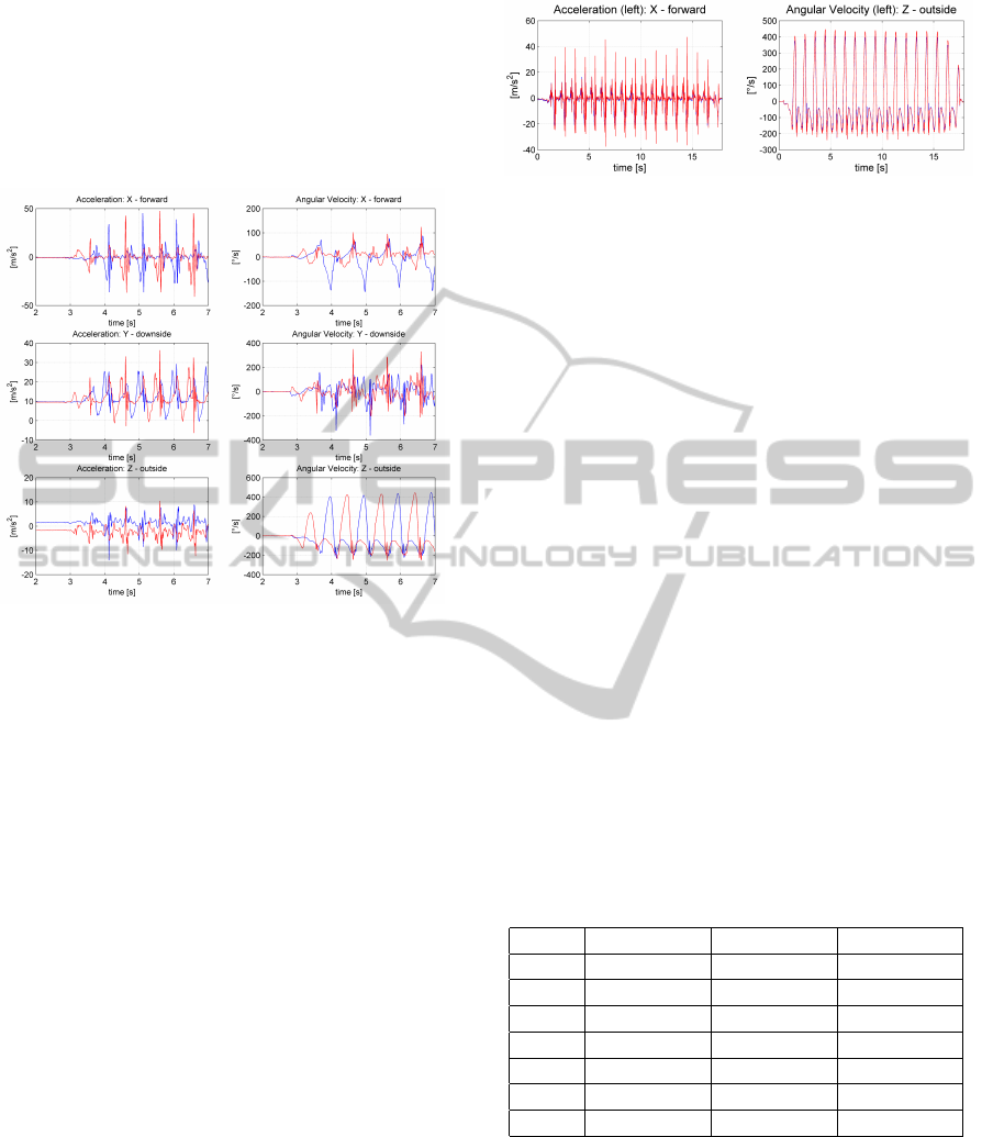
Figure 2: Raw data of Xsens sensors (left - blue, right - red).
2.4 Preprocessing
The preprocessing includes four steps:
1. Reading, reorganizing and renaming the experi-
mental raw data of both systems: As a result of
that step, acceleration and angular velocity of ev-
ery passage are collected in one dataset. The three
components (x,y,z) of them are oriented along the
correspondent axes of the inertial coordinate sys-
tem (compare figures 1 and 2).
2. Attuning the signals of both sensor types to com-
mon sampling intervals given by the lower sam-
pling rate (mostly 100 Hz): The smaller dataset
is interpolated to reach the same length and time
resolution of the larger dataset.
3. Synchronizing the signals of both sensor types us-
ing correlation between the angular velocities ω
z
:
The distance between the cross correlation of the
signals of both systems and the auto correlation of
Shimmer signals is calculated and applied to shift
the Shimmer signals.
4. Cutting the resting phase before and after the mo-
tion, so that the movement signals are integrated
(forward velocity v
x
is positive).
The results of preprocessing are presented in figure 3.
Figure 3: X-axis of acceleration and z-axis of angular ve-
locity after preprocessing (blue Shimmer, red Xsens).
2.5 Discussion
After preprocessing 103 out of 144 datasets were ex-
tracted for further investigation. 41 datasets were
rejected because of the missing or erroneous data.
Xsens data mark incorrect values with ”NaN”, which
were removed manually before preprocessing.
There is no substantial difference between the
measurements of acceleration and angular velocity of
Shimmer and Xsens sensors. Caused by the chosen
sensitivity of ±1.5g the Shimmer acceleration signals
are limited at ±20m/s
2
. Higher peaks are cut.
Table 2 summarizes the dependencies between the
walking velocity, the covered distance and the cho-
sen speed. Analogue to that the number of strides are
shown. The dependencies coincide with our expec-
tation. The stride number is greater, the higher the
pace and the longer the distance, but it rises under-
proportionally with the distance. Ergo, the stride
length is larger and the mean velocity higher, the
longer the distance. The measured velocity corre-
sponds to the chosen speed. These facts have been
evidenced by the measured gait sequences.
Table 2: Mean velocity in m/s (std) and mean number of
strides (std).
slow normal fast
20 m 1.05 (0.1) 1.25 (0.08) 1.5 (0.12)
40 m 1.17 (0.08) 1.36 (0.13) 1.53 (0.1)
60 m 1.21 (0.09) 1.4 (0.08) 1.71 (0.13)
20 m 16.2 (4.6) 14.2 (3.8) 13.2 (3.4)
40 m 25.7 (8.5) 26.6 (8.3) 22.5 (5.7)
60 m 40.8 (13.0) 37.7 (10.9) 33.4 (8.3)
While the standing before and after the acceleration
sensors measure only the gravity acceleration g =
−9.81m/s. If the alignment of the sensors in the sagit-
tal plane is ideal, a
x
and a
z
are zero while a
y
is equal
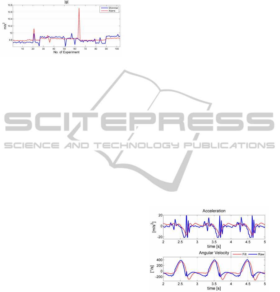
to g. Two mentionable types of errors are:
- The norm of the acceleration vector differs from g
(see figure 4). It was calculated and averaged in an
interval of 1 s before motion.
- The observed a
x
and a
z
differs from zero, i.e., the
BIOSIGNALS2014-InternationalConferenceonBio-inspiredSystemsandSignalProcessing
266
gravity vector participates to these components.
Figure 4: Measured vector of gravitation before motion rep-
resenting the problem of calibration and sensor drift.
3 METHODS
The sensors are fixed to the lower shank above the
ankle and move all the time with the shanks changing
their orientation. To calculate the covered distance
only the component in the direction of motion is of
interest. Following the vector of acceleration has
to be projected to the horizontal component a0
x
in
the sagittal plane (of inertial coordinate system). In
principle, different approaches are possible:
- To calculate all kinematic features including the
forward motion from the sampled data. The mathe-
matical background is given in (Loose and Orlowski,
2012), but the accumulated error is growing with the
duration of motion.
- To estimate the orientation of the sensor coordinate
system (Xsens), to project the acceleration on the x-
axis of the inertial coordinate system and to integrate
it twice to get the covered distance s.
- To estimate the vector of acceleration a0, of velocity
v0 and of distance s0 as well as the angular velocity
ω and the orientation matrix R using the Kalman
filter technique (Welsh, 1996)
- To approximate the needed component a0
x
using
one or two components of the acceleration.
All approaches need additional and/or apriori knowl-
edge about the motion, e.g. initial and intermediate
state information or integral properties of the process:
- There is no motion before and after measurement,
i.e. initial and final velocity is equal to zero. The
integral of acceleration over the whole time is equal
to zero, too.
- The motion is straight forward, i.e. the forward
velocity is always greater than zero (v >= 0) and,
following, the velocity of the ankle is v > v
min
> 0
during motion.
- The vertical motion of the ankle and the declination
of the shank from the vertical are relatively small
(with regard to the horizontal motion).
- The motion is nearly periodic and stride-based.
- The horizontal component of the ankle is v
x
>= 0,
y = y
min
before and after stride for each leg.
In this paper only the measured components a
x
and ω
z
are used to calculate the covered distance. The
simplification is based on the assumption that the dec-
lination of the shank from the vertical is small. In
that case the gravity can be eliminated and the verti-
cal acceleration neglected. The DC part of a0 and ω
is eliminated by high pass and the noise by low pass
filtering. The integral of the AC part over the whole
motion (each stride) must be zero because of the pe-
riodicity of motion (stance phase of each leg).
Two different methods are investigated: whole
signal and stepwise integration (stride).
Both approaches start with band pass filtering of
the acceleration a
x
and angular velocity ω
z
. The
stop and pass frequencies of the low pass were set
to 20 and 10 Hz. The influence of the filter param-
eters, especially the pass and stop band of the high
pass, were investigated. The high pass is used to
eliminate systematic offset of measurement and the
gravity. The pass frequency must be less than min-
imum stride frequency (∼ 0.7Hz). The following
pairs of stop and pass frequencies (in Hz) were tested:
[0.25,0.6],[0.2, 0.5],[0.15,0.3], [0.1,0.2],[0.05, 1].
The best results were achieved using the second
pair. The results of optimal filtering are shown in
figure 5.
Figure 5: Raw and filtered signal of a
x
and ω
z
.
Whole Signal Integration (WSI)
- Integrating a
x
using an IIR-filter with the kernel
[0.5 0.5]/[1 -1] (trapezoid rule).
- Adding an offset min(v
x
) to v
x
, so that v
x
≥ 0.
- Calculating s
x
from v
x
using the same filter.
Stepwise Integration (SWI)
- Detecting the feature points representing the begin
and the end of a stride, for left and right leg, respec-
tively.
SimpleAlgorithmsfortheDeterminationoftheWalkingDistancebasedontheAccelerationSensor
267
- Calculating the covered distance s
x
for any stride
by integrating a
x
, adding an offset to v
x
, so that
v
x
> v
min
> 0; where v
min
= 0.15 ∗ mean(v
x
), calcu-
lating s
x
integrating v
x
.
- Accumulating all single distances to the covered
distance s.
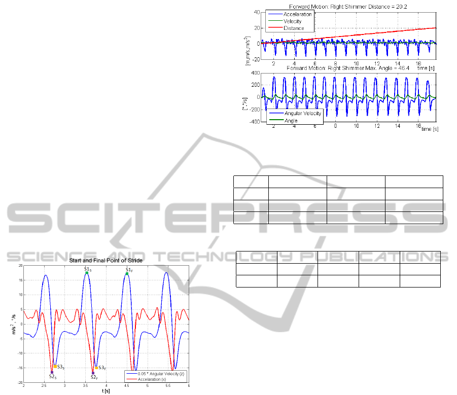
Three variants for the detection of strides were
investigated (see figure 6):
Method S1. The maximum angular velocity ω
z
is the
point characterizing the start/final point of any stride.
These points lie a bit after the maximum velocity v
x
and before the maximum deceleration −a
x
.
Method S2. The maximum deceleration −a
x
is the
point characterizing the start/end point. These points
lie a bit before the terminal contact (TC).
Method S3. The swing phase of a stride is defined
by TC to the initial contact (IC) of the foot on the
ground. Following, the stance phase is defined by IC
and TC. Algorithms to detect these points are found
in (Orlowski and Loose, 2013; Greene et al., 2010).
Here any stride lasts from one TC to next one.
Figure 6: Start and final point of stride for methods S1-S3.
4 RESULTS
Figure 7 shows typical curves of the kinematic char-
acteristics: linear acceleration, velocity and displace-
ment, angular velocity and angle.
The covered distance is the most important calculated
value characterizing the quality of algorithms. The
”relative distance” d
rel
is a measure of that goodness:
d
rel
= d
calc
/d
abs
.
The mean over all calculations after elimination of
obvious outliers is 0.97 ± 0.09σ, the relative error is
3% ± 9%. That feature depends on the walking dis-
tance as well as on the chosen speed (see table 3).
The best result is achieved in the case of normal
pace (0.97 ± 0.07σ). For slow motion the distance is
overestimated, while for the fast it is underestimated.
The reason is that the algorithm was adjusted for nor-
Figure 7: Kinematic characteristics for one leg of a subject.
Table 3: Relative distance - mean (std).
slow normal fast
20 m 1.1 (0.1) 0.97 (0.07) 0.89 (0.1)
40 m 0.96 (0.07) 0.96 (0.1) 0.89 (0.08)
60 m 1.05 (0.08) 1 (0.07) 0.93 (0.09)
Table 4: Relative distance on method.
method A1 S1 S2 S3
mean 1.04 0.8 0.98 0.98
std 0.1 0.09 0.1 0.1
mal speed and 20 m distance.
Table 4 shows that all four algorithms work
well. The algorithm A1 (WSI) overestimates the dis-
tance (4%(±10%)) while the SWI algorithms (S2,
S3) are comparable and underestimate the distance
(2%(±10%)). The underestimation can be easily
compensated adjusting the parameter v
min
.
Comparing the calculated distances based on the
data captured from Shimmer and Xsens sensors,
Shimmer data returns shorter distances than Xsens
data (37.0 m vs. 39.6 m for left and 35.2 m vs. 37.7
m for right side). The difference between both sen-
sor types is caused by the limitation of ±1.5g set for
Shimmer sensors. The difference between the left and
the right side can be explained by the fact that the
subjects start motion with a half stride of one leg and
finish with a half stride of the same or the other leg.
The inter class variability has been investigated.
There are some differences which are explainable by
the different number and types of datasets, i.e. all
distances and speeds are included into the evaluation.
There are dependencies between the relative distance
and the velocity as well as the number of strides and
the calculated distance.
Figure 8 shows results for all datasets with respect
to the covered distance. The relative distance is pre-
sented. There is a relatively high number of outliers.
Strides greater than 2 m or less than 0.5 m are not
existent during walking of healthy adults.
BIOSIGNALS2014-InternationalConferenceonBio-inspiredSystemsandSignalProcessing
268
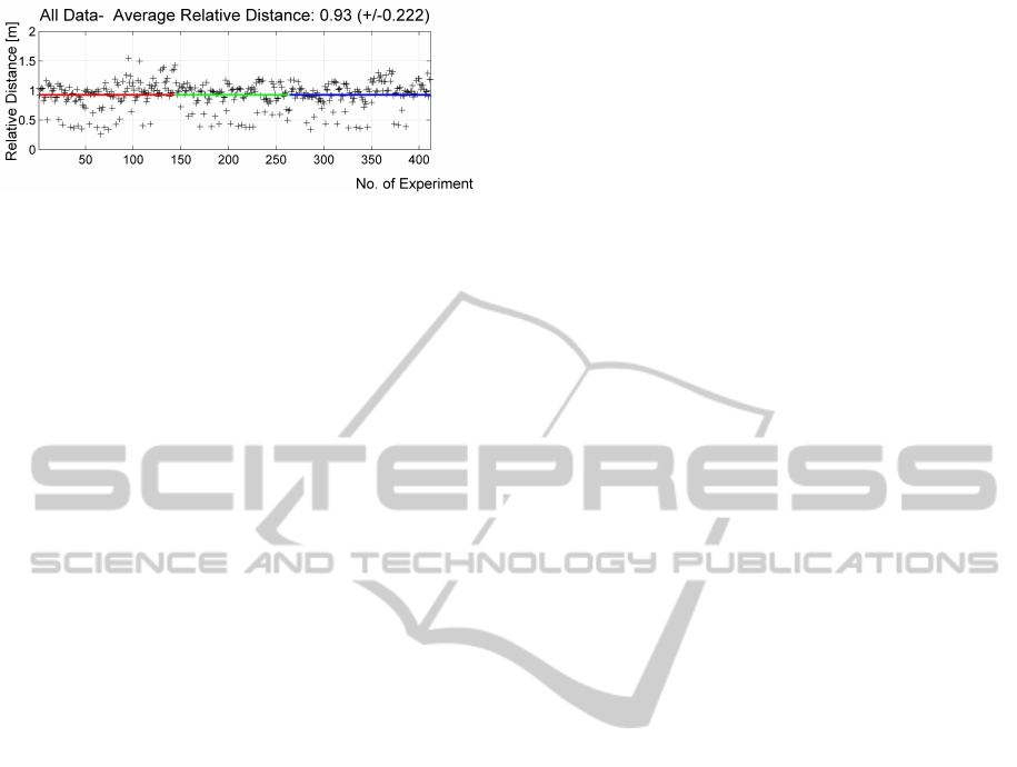
Figure 8: Average relative distance sorted by distance (20
m - red, 40 m - green, 60 m - blue).
5 DISCUSSION AND
CONCLUSIONS
The purpose of this investigation was to develop a
simple algorithm for the calculation of the distance
covered while walking. Simplicity in that case means
that there is no information about the orientation of
the sensor. The algorithm is implementable on mo-
bile devices like mobile phones. The investigated al-
gorithms were based on the ”horizontal” components
a
x
and ω
z
. Two different approaches, were imple-
mented and compared (WSI vs. SWI). Statistically all
methods work well. The mean of the relative distance
is 0.97, but the variance is not negligible σ = 9%.
The quality of the results depend on the speed of mo-
tion. A large number of outliers were determined and
the reasons must be analyzed. The source of errors
caused by calibration can be reduced, i.e. by recali-
brating sensors any time before every subject.
The algorithms will be improved in the future in-
cluding e.g. the vertical component of the accelera-
tion, the declination of the sensor at the beginning and
during the motion. A comparison with Kalman filter
approaches and the determination of the orientation
delivered by Xsens sensors have to be conducted.
Further experiments such as walking on a tread-
mill at different speeds are planned. It seems to be
that simple algorithms based on acceleration and an-
gular velocity can satisfy everyday needs.
REFERENCES
Bai, L., Pepper, M., Yana, Y., Spurgeon, S., and Sakel,
M. (2012). Application of low cost inertial sensors
to human motion analysis. IEEE InternationalInstru-
mentation and Measurement Technology Conference
(I2MTC), pages 1280 – 1285.
Bebek, O., Suster, M., Rajgopal, S., Fu, M., Huang, X.,
Cavusoglu, M., Young, D., Mehregany, M., van den
Bogert, A., and Mastrangelo, C. (2010). Personal nav-
igation via high-resolution gait-corrected inertial mea-
surement units. IEEE Transactions on Instrumenta-
tion and Measurement,, 59:3018–3027.
Bird, J. and Arden, D. (2011). Indoor navigation with foot-
mounted strapdown inertial navigation and magnetic
sensors. IEEE Wireless Communications, pages 28–
35.
Cavallo, F., Sabatini, A. M., and Genovese, V. (2005). A
step toward gps/ins personal navigation systems: real-
time assessment of gait by foot inertial sensing. In-
ternational Conference on Intelligent Robots and Sys-
tems (IROS 2005), pages 1187 – 1191.
Feng, S. and Law, C. L. (2002). Assisted gps and its im-
pact on navigation in intelligent transportation sys-
tems. Proceedings of The IEEE 5th International Con-
ference on Intelligent Transportation Systems, pages
926–931.
Greene, B. et al. (2010). An adaptive gyroscope-based algo-
rithm for temporal gait analysis. Med Biol Eng Com-
put, 48:1251–1260.
Liu, T., Inoue, Y., Shibata, K., and Shiojima, K. (2012). A
mobile force plate and three-dimensional motion anal-
ysis system for three-dimensional gait assessment.
IEEE Sensors Journal, 12(5):1461 – 1467.
Loose, H. and Orlowski, K. (2012). Measurement of human
locomotion: Evaluation of low-cost kinect and shim-
mer sensors. In: MSM 2012, The 8th International
Conference Mechatronics Systems and Materials, 8.
Orlowski, K. and Loose, H. (2013). Evaluation of kinect
and shimmer sensors for detection of gait parame-
ters. Proceedings of BIOSIGNALS 2013, Int. Confer-
ence on Bio-Inspired Systems and Signal Processing,
Barcelona, Spain, 11-14 Feb. 2013, pages 157–162.
Pratama, A. R., Widyawan, and Hidayat, R. (2012).
Smartphone-based pedestrian dead reckoning as an in-
door positioning system. Proceedings of International
Conference on System Engineering and Technology,
pages 1–6.
Roetenberg, D., Luinge, H., and Slycke, P. (04/2009).
Xsens mvn: Full 6 dof human motion tracking using
miniature inertial sensors. XSENS TECHNOLOGY,
WHite Paper.
Shimmer Research, e. (2011). Wireless sensing solution.
http://shimmer-research.com.
Suh, Y. S. and Park, S. (2009). Pedestrian inertial navigation
with gait phase detection assisted zero velocity updat-
ing. Proceedings of the 4th International Conference
on Autonomous Robots and Agents, pages 336–340.
Welsh, G. (1996). SCAAT: Incremental Tracking with In-
complete Information. PhD thesis, University of North
Carolina.
Xsens Technologies B.V., e. (2012). MTw User Manual -
MTw Hardware, MT Manager, Awinda Protocol (Re-
vision E). Xsens Technologies B.V., Enschede, NL,
fifth edition.
SimpleAlgorithmsfortheDeterminationoftheWalkingDistancebasedontheAccelerationSensor
269
