A Revisited Model for the Real Time Trafﬁc Management

Astrid Piconese

, Thomas Bourdeaud’Huy

, Mariagrazia Dotoli

and Slim Hammadi

DEE, Department of Electrical Engineering and Information Science, Politecnico di Bari, Bari, Italy

LAGIS, Laboratoire d’Automatique, G´enie Informatique et Signal,

Ecole Centrale de Lille, Lille, France

Keywords:

Railway Systems, Real-time Optimization, Regional Networks, Single-track, Centralized Trafﬁc Control,

Linear Programming.

Abstract:

The real-time trafﬁcmanagement allow to solve unexpected disturbances that occur along a railway line during

the normal developement of the trafﬁc. The original timetable is restored through the rescheduling process.

Despite the increase of real-time decision support tools for trains dispatchers that enable a better use of rail in-

frastructure, real-time trafﬁc management received a limited scientiﬁc attention. In this paper, we deal with the

real time trafﬁc management for regional railway networks, mainly single tracks, in which a centralized trafﬁc

control system is installed. The rescheduling problem is presented as a Mixed Integer Linear Programming

Model which resolution allows to carry out the rescheduling process in a very short computational time.

1 INTRODUCTION

A railway system is a complex system with many

interacting processes that depend on technical de-

vices, human behavior, external environment, and

therefore contains many risks of disturbances. The

usual method how railways manage their trafﬁc per-

formance is through a carefully designed plan of op-

erations, deﬁning several months in advance routes,

orders and timing for all trains. This process, called

off-line timetabling, is followed by a real-time traf-

ﬁc management which consists in managing distur-

bances that may occur during the ordinary function-

ing of the network.

Once a delayed train deviates from its original

schedule, it may propagateits delay to other trains due

to infrastructure, signaling or timing conﬂicts. Ma-

jor disturbances may inﬂuence the off-line plan of op-

erations that should be subject to short-term adjust-

ments in order to minimize the negative effects of the

disturbances. Possible trafﬁc control actions include

changing dwell times at scheduled stops, changing

train speeds along lines, or adjusting train orders at

junctions, stations and passing points. Other control

actions involve major modiﬁcations such as changing

train routes or even canceling scheduled train jour-

neys. The main goal of the real-time dispatching is

to minimize trains delays, while satisfying the traf-

ﬁc regulation constraints, and ensuring compatibility

with the current position of each train, see (D’Ariano,

2008).

In this paper we deal with real-time trafﬁc control

problem for a regional single-track railway where an

operating system called Centralized Trafﬁc Control

(CTC) is installed. The CTC provides a centralized

control for signals and switches within a limited ter-

ritory, controlled from a single control console. The

command is carried out by the Train Dispatcher (TD).

The train dispatcher observes the status of the ter-

ritory – i.e. occupation of line sections, location of

trains, etc. – in a continuous manner and collects in-

formation; meanwhile, he communicates with the up-

per level decision-makers and the staff in the territory

in order to exchange decisions taken. In case of an un-

planned event and emergency he takes a decision and

makes necessary actions in accordance with the rules

and regulations pre-deﬁned by the railway authority,

see (

Ismail, 1999).

The TD may beneﬁt from appropriate decision

support system, such as scheduling algorithms, to per-

form a real-time simulation and evaluation of traf-

ﬁc under disturbances in order to quickly reschedule

train movements and to reduce delays from a global

perspective.

It is important to ﬁnd a good compromise between

the solution quality, the time horizon of the trafﬁc

prediction, and the computational effort. If a short

time horizon is adopted, only few trains, and few con-

ﬂicts, can be detected and solved with short computa-

tion times. On the other hand, a longer time horizon

139

Piconese A., Bourdeaud’huy T., Dotoli M. and Hammadi S..

A Revisited Model for the Real Time Trafﬁc Management.

DOI: 10.5220/0004869701390150

In Proceedings of the 3rd International Conference on Operations Research and Enterprise Systems (ICORES-2014), pages 139-150

ISBN: 978-989-758-017-8

 2014 SCITEPRESS (Science and Technology Publications, Lda.)

leads to a larger number of trains running in the sys-

tem, in order to eliminate completely the propagation

of the disturbance. There is a tradeoff between the

size of the time horizon of trafﬁc prediction (bigger

time horizon meaning better quality) and the compu-

tational time. In fact, in a small time horizon the real-

time dispatching does not take into account conﬂict-

ing trains outside the time horizon. On the other hand,

a conﬂict arising far in the future may not be as rele-

vant as a closer conﬂict, since other unforeseen events

could still affect the further conﬂict, see (D’Ariano,

2008). In a small time horizon, the computational

time is smaller because datas are limited.

Usually the train dispatcher reschedules the in-

volved trains, depending on the known duration of

the disturbance. He bases his decisions on his own

knowledge, resolving a conﬂict at a time when it oc-

curs, and then manually rebuilds the timetable, with

a considerable waste of time and no certainty that its

decisions will lead to an optimal solution.

Building on the formalism given in (Dotoli et al.,

2013), we present a model that solves the reschedul-

ing problemforregionalpassenger transport networks

with stations of equal importance, where the CTC sys-

tem is installed. We formulate the problem as a Mixed

Integer Linear Programming Problem (MILP).

In the original model the new timetable after the

disturbance is obtained by minimizing train delays

in all the stations programmed in their path, while

considering constraints regarding travel times, stop

times at stations, safety standards and network capac-

ity. The model is applied to a limited time horizon

that is choosen by the analyst. In order to solve con-

ﬂicts that may occur in the rescheduled timetable af-

ter the time horizon, an iterative heuristic algorithm is

applied. The heuristic algorithm solves a conﬂict at

the time when it occurs; priority is given to the train

with the highest traveling time, namely the longest

presence on the line. The computational time for

limited time horizons is of the order of seconds, but

the heuristic algorithm requires an elevated computa-

tional time that depends on the number of trains and

the complexity of the raiway line. The methodology

provides a decision support system to the train dis-

patcher that has to take decisions in order to restore

trafﬁc and limit inefﬁciencies for passengers.

We adapt the previous methodology to regional

networks mainly made of single tracks and take into

account the constraints imposed by the railway infras-

tructure and the time constraints imposed by the ini-

tial schedule.

The revised model solves all conﬂicts that arise

along the railway line after the occurrence of the

disturbance; the heuristic algorithm is therefore no

longer applied. The rescheduled timetable is estab-

lished in a shorter time, then discomfort for passen-

gers is restricted and the quality of the transport ser-

vice is increased.

To show its effectiveness, we study the problem

in a particular section of a railway network located in

Southern Italy, see (FSE - Ferroviedel Sud Est, 2013).

The FSE network is constituted by single tracks with

few double track segments and in some stations only

one train can stop or pass through.

The paper is organized as follows. In Section 2 we

present the problem formalization. In Section 3 the

mathematical model for the resolution of the problem

is proposed. In section 4 we present the application

of the model to the case study of the FSE railway net-

work. Finally, Section 5 contains some concluding

remarks and suggestions for further research.

2 PROBLEM FORMALIZATION

2.1 Initial Scheduling

Deﬁnition 1 (Railway Network). A railway network

is deﬁned by a set of segments on which trains runs.

Segment (b

): A segment b is a railway section

between two points. We deﬁne by B =

, b

, . . . , b

} = {b

}

i∈[[1,B]]

the set of segments.

B denote the cardinality of the set B. The set of

segments is partitioned into the subset B

corre-

sponding to segments into a station, and B

corre-

sponding to the subset of rail connections outside

stations.

Track (v

): Let b be a segment ∈ B. We deﬁne by

= {v

, v

, . . . v

} = {v

}

j∈[[1,V

]]

the set of par-

allel tracks in b. The set of all tracks in the railway

network is denoted by V. V and V

denote respec-

tively the cardinality of V and V

for a given seg-

ment b. Given a track v ∈ V, we denote by b

its

corresponding segment.

Circulations in a railway network are deﬁned by a

set of trains. Train’s path is made of an ordered set of

movements.

Deﬁnition 2 (Trains and Movements). We assume

that the train’s length is compatible with the length

of all tracks that compose the railway line. Trains are

thus deﬁned as follows.

Train (t

): The set of trains using the railway

network is denoted as T = {t

, . . . , t

} =

}

k∈[[1,T]]

. T denotes the cardinality of T.

Train Direction (d

): Each train is deﬁned by a di-

rection parameter expressing the position of its

ICORES2014-InternationalConferenceonOperationsResearchandEnterpriseSystems

140

destination station. Let t be a train ∈ T. We de-

note by d

= 0 the direction of a train which head

goes to the north (a.k.a. “even trains”) of the rail-

way line, and d

= 1 of a train running to the south

(a.k.a. “odd trains”).

Movement (µ

): A movement indicates the request

for a track by a train. Let t be a train ∈ T. We de-

ﬁne by M

= {µ

, µ

, . . . , µ

} = {µ

}

p∈[[1,M

]]

the

ordered set of movements of train t. M

denotes

the cardinality of M

. µ

first

= µ

and µ

last

= µ

denote respectively the ﬁrst and the last element

in M

. We deﬁne by M the set of all movements

on the railway line and by M

last

the set of the last

movements of each train.

Train movements are deﬁned by several parameters.

Movement Direction: All movements µ of a train t

share the same direction as their train, denoted as

∀t ∈ T, ∀µ ∈ M

, d

= d

(1)

Track and Segment of a movement (b

, v

): Each

movement µ of a train is scheduled in an unique

segment b

∈ B. We denote by M

the set of

movements scheduled in the same segment b ∈ B.

Each movement µ ∈ M must be scheduled in a

track of the segment b

, denoted as v

, according

to the following constraint:

∀t ∈ T, ∀µ ∈ M

, v

∈ V

(2)

Reference Schedule Times (α

ref

, δ

ref

, γ

ref

): Each

train movement µ is associated to reference times

corresponding to its initial schedule. Let t ∈ T

be a train and µ ∈ M

one of its movements.

We deﬁne three reference times α

ref

, δ

ref

, γ

ref

∈ N,

where:

- α

ref

is the starting time of µ as established in the

initial schedule, expressed in minutes taking as

reference a time T

∈ N.

- δ

ref

is the duration of µ (expressed in minutes)

if it occurs in a rail connection, i.e. the mini-

mum running time deﬁned in the initial sched-

ule. This quantity is equal to 0 if the movement

occurs in a station. Formally:

∀t ∈ T, ∀µ ∈ M

, b

∈ B

⇒ δ

ref

= 0 (3)

- γ

ref

is the duration of a movement µ (in minutes)

if it occurs in a station, i.e. the minimum stop-

ping time deﬁned in the initial schedule. This

quantity is equal to 0 is the movement occurs in

a rail connection. Formally:

∀t ∈ T, ∀µ ∈ M

, b

∈ B

⇒ γ

ref

= 0 (4)

Using such notations, the time interval during

which a movement µ reserves its track can be ex-

pressed as [[α

ref

, α

ref

+δ

ref

+γ

ref

= β

ref

]]. Two con-

secutive movements must be scheduled according

to these intervals, thus we have:

∀t ∈ T, ∀p ∈ [[1, M

[[, (5)

ref

p+1

= α

ref

+ δ

ref

+ γ

ref

In order to reduce the size of the initial problem we

could use only one variable ζ = γ + δ to represent

movements duration. However, even if such formu-

lation would reduce the number of initial variables,

the size of the problem after the presolve phase would

remain unchanged, since modern solvers are able to

detect such redundant variables. For clarity, we de-

cided thus to keep using two different variables γ and

δ to represent movementduration respectively in a rail

connection and in a station.

Deﬁnition 3 (Security Constraints). Since several

trains run at the same time on a railway network, sev-

eral constraints must be veriﬁed to ensure the security

of circulations.

Track Occupation Constraints: A track cannot be

occupied by two trains at the same time. Such re-

striction can be expressed formally by constrain-

ing any pair of movements using the same track to

be scheduled on disjoint timing intervals:

∀t

∈ T, ∀µ

∈ M

, ∀µ

∈ M

= v

⇒ [[α

ref

, β

ref

]] ∩ [[α

ref

, β

ref

]] = ∅ (6)

Safety Times (∆

, ∆

): The safety time is the sepa-

ration time that has to elapse between two move-

ments µ

, µ

on the same track (i.e. between a

train leaving one track and another one entering

the same track). We denote by ∆

∈ N the safety

time required if trains meet and ∆

∈ N if one

train is following the other one. ∆

and ∆

are

expressed in the same time units as γ

ref

and δ

ref

These time delays must occur between the end of

the ﬁrst movement (denoted as β

ref

) and the start

of the otherone (denoted as α

ref

). Formally, safety

time constraints can be expressed as follows:

∀b ∈ B, ∀µ

, µ

∈ M

= v

∧ d

= d

⇒

(

ref

≥ β

ref

+ ∆

∨ α

ref

≥ β

ref

+ ∆

(7)

= v

∧ d

6= d

⇒

(

ref

≥ β

ref

+ ∆

∨ α

ref

≥ β

ref

+ ∆

(8)

ARevisitedModelfortheRealTimeTrafficManagement

141

Note such constraints renforce the constraint (6)

since they induce a separation delay between the

time intervals of two movements on the same

track.

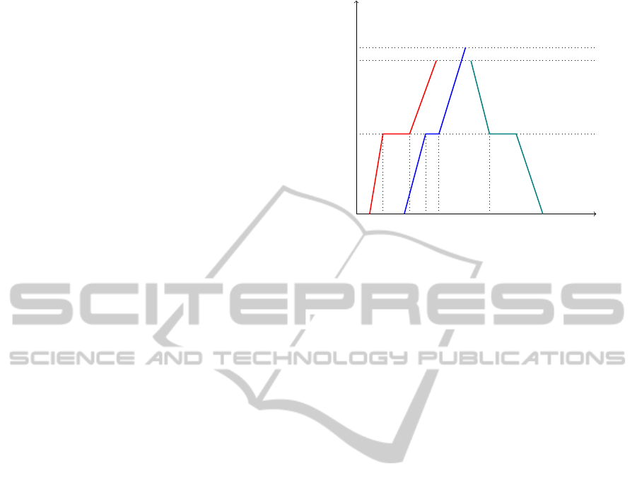
A rail transport service on a railway line is graph-

ically represented by a cartesian graph, representing

the safety constraints.

Graphic Timetable: The graphic timetable is a

cartesian graph that represents the situation of a

railway schedule for a day, see (Vicuna, 1989).

The diagram shows all movements, scheduled and

safety times.

The time line is plotted on the x axis. The rail-

way line (space) is plotted on the y axis. Inside

stations, tracks are represented by dashed lines

parallel to the x axis. Trains are represented by

an oblique broken line which orientation indicates

train direction. For instance, train lines are ori-

ented from bottom to up for even trains that travel

from south to north (i.e. to the station on the upper

end of the y axis).

Figure 1 represents the graphic timetable of three

trains t

, t

and t

. Train t

is directed to the

South, while t

and t

travel in the opposite di-

rection. The railway line is made of 5 segments:

single-tracked stations b

and b

, double-tracked

station b

and single-tracked rail connections b

and b

. Track sets for the ﬁve segments are de-

ﬁned by: V

= {v

}, V

= {v

}, V

= {v

, v

= {v

}, V

= {v

}. Train’s paths are deﬁned

by sets: M

= (µ

, µ

), M

= (µ

, µ

= (µ

, µ

). All trains cross station b

that

is single-tracked. As shown, safety times are ap-

plied when two trains occupy the same track of a

segment. ∆

is the safety time that has to elapse

between the end of the movement µ

and the be-

ginning of µ

, where t

and t

travel in the same

direction. ∆

is the safety time that has to elapse

between the end of µ

and the beginning of µ

where t

and t

travel in opposite direction.

2.2 Disturbances Issues

When a disturbance occurs along the railway net-

work, that compromises the normal trafﬁc operation,

a rescheduling process must be accomplished taking

into account time constraints imposed by the initial

schedule.

Deﬁnition 4 (Disturbance). A disturbance denotes

the deviation of a train t

∈ T from its original sched-

ule due to an unforeseen situation, concerning one of

its movements µ

∈ M

time

Segment

ref

∆

Figure 1: Graphic Timetable.

Disturbance Duration and Reference Time:

When a disturbance occurs, a disturbance refer-

ence time T

is deﬁned as the ﬁrst time on which

the disturbance has an impact on the schedule of

the others trains, i.e. the reference ending time of

the disturbed movement. If only one disturbance

affects one movement µ

∈ M

of a train t

along

the railway line, T

is deﬁned as:

= β

ref

We denote by ∆

the disturbance duration ex-

pressed in minutes. The impact of a disturbance

on the movement is expressed by an increase of

the value of parameter δ or γ depending on the na-

ture of the segment on which the disturbance oc-

curs. For instance, if b

∈ B

, δ

′

= δ

ref

+ ∆

Conversely, if b

∈ B

, γ

′

= γ

ref

+ ∆

If two independent disturbances affect two differ-

ent trains along the line, T

is deﬁned as the mini-

mum ﬁnal time of movements affected by the per-

turbation. Let t

and t

be two trains affected by

the disturbance. Let µ

∈ M

and µ

∈ M

the perturbed movements. T

is deﬁned as:

= min

ref

, β

ref

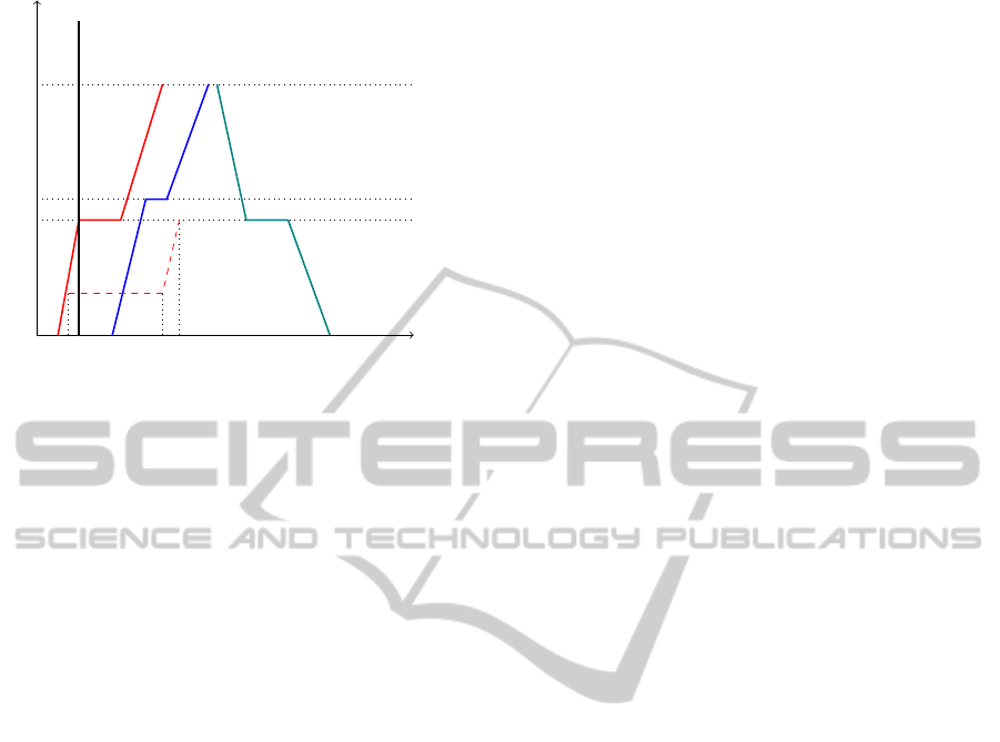
Figure 2 represents a railway line made of three

station (b

, b

and b

) and two single-tracked rail

connections (b

and b

). A disturbance occurs in

and affects only the movement µ

∈ M

. Ref-

erence time T

coincides with β

ref

. The dashed

line shows the movement µ

after the end of the

rescheduling process. The recheduled crossing

time δ

ef f

is equal to the reference time δ

ref

in-

creased by the disturbance duration ∆

. The ef-

fective path of movement µ

interferes with the

ICORES2014-InternationalConferenceonOperationsResearchandEnterpriseSystems

142

time

Segment

ref

≡ β

ref

eff

∆

Figure 2: Disturbance of t

path of another movement in the segment b

that

has to be rescheduled.

Effective Schedule Times: In order to take into ac-

count the effect of the disturbance on the subse-

quent movements on the railway network, we in-

troduce for any movement its effective scheduled

times denoted by α

eff

, δ

eff

and γ

eff

∈ N. Obviously,

movements which ﬁnal date β is scheduled before

are not altered. Formally:

∀t ∈ T, ∀µ ∈ M

s.t.β

ref

≤ T







eff

= α

ref

eff

= δ

ref

eff

= γ

ref

(9)

Effective Time Constraints: These new scheduled

times must allow to absorb the perturbation by

delaying the initial reference times, according to

their respective segment types, following con-

straints (3) and (4). Formally, these previous

equations become:

∀t ∈ T, ∀µ ∈ M

s.t.β

ref

> T

∈ B

⇒







eff

≥ α

ref

eff

= δ

ref

= 0

eff

≥ γ

ref

(10)

∈ B

⇒







eff

≥ α

ref

eff

≥ δ

ref

eff

= γ

ref

= 0

(11)

Effective schedule time must also obviously fol-

low the sequencing constraint (5) and safety con-

straints (6), (7) and (8).

Time Horizon (H): The time horizon H is the term

planning in which the rescheduling operations are

carried out. It consists of a given number of

timetable minutes in which a given number of

trains are scheduled on the railway line. Move-

ments after the time horizon are not taken into ac-

count in the rescheduling process, even if they be-

long to trains of which ﬁrst movements belong to

the time horizon.

Of course, depending on the density of trafﬁc at

the time of the disturbance, and its duration, the num-

ber of disturbed movements can vary considerably.

In this paper, we consider all the scheduled move-

ments of the day but one of our objective functions

can be designed to minimize the number of resched-

uled trains.

In the following section, we present the Mixed In-

teger Linear Programming Model that allows to solve

the rescheduling problem, i.e. to give a value to each

effective scheduled time while respecting the safety

constraints and optimizing practical criteria.

3 MATHEMATICAL MODELING

3.1 Decision Variables

We introduce additional variables and constants used

to express the problem in a linear way.

- X

µ,v

∈ {0, 1}

M×V

is the variable that identiﬁes the

track v on which a movement µ occurs. X

µ,v

ϕ(v = v

) where the function ϕ(C) is the indica-

tor ϕ(C) = 1 if the condition C is veriﬁed, 0 oth-

erwise.

- X

before

,µ

∈ {0, 1}

M×M

is the variable that charac-

terizes the chronological order of two movements

, µ

if they use the same segment. X

before

,µ

ϕ(µ

is scheduled before µ

- X

delay

∈ {0, 1}

is the variable that specify if a

train t deviates from its original schedule and is

therefore delayed. X

delay

= ϕ(β

ef f

> β

ref

- X

delay

∈ {0, 1}

is the variable that specify if a

movement µ deviates from its original schedule

and is therefore delayed. X

delay

= ϕ(β

ef f

> β

ref

- B ∈ N is a sufﬁciently large positive constant.

- H ∈ N is a parameter that deﬁnes the size of the

time horizon.

By deﬁnition, the previous decisions variables are

subject to constraints characterizing their physical

sense.

• Any movement can only be scheduled on one

track of its segment, consequently:

∀µ ∈ M,

∑

v∈V

µ,v

= 1 (12)

ARevisitedModelfortheRealTimeTrafficManagement

143

• Two movements scheduled on the same segment

must be ordered:

∀b ∈ B, ∀µ

, µ

∈ M

, (13)

before

,µ

+ X

before

,µ

= 1

Safety constraints presented above must be ex-

pressed using those variables in linear way.

3.2 Linearization of Safety Constraints

Security constraints (6), (7) and (8) are expressed

through the use of additional variables and constraints

in order to obtain a linear formulation.

3.2.1 Tracks Occupation Constraints

Constraint (6) speciﬁes that a track v cannot be oc-

cupied by several movements at the same time. Con-

straints (7) and (8) express a separation delay must

elapse between two movements occupying the same

track. These conditions can be expressed by the fol-

lowing equations:

∀b ∈ B, ∀µ

, µ

∈ M

s.t. d

= d

, ∀v ∈ V

, (14)

eff

− α

eff

+ ∆

≤ B·



3− X

before

,µ

− X



∀b ∈ B, ∀µ

, µ

∈ M

s.t. d

6= d

, ∀v ∈ V

, (15)

eff

− α

eff

+ ∆

≤ B·



3− X

before

,µ

− X



Note for any pair of movements µ

, µ

, two in-

stances of the previous equations (14) and (15) are

considered in the mathematical model depending of

the the order of movements: (µ

, µ

) or (µ

, µ

The previous equation expresses that if two move-

ments µ

, µ

occurs on the same track, and if X

before

,µ

1, then µ

must end before the start of µ

. If X

before

,µ

= 0

or µ

and µ

do not occur in the same track, equation

(14) and (15) are trivially veriﬁed.

The disjunction operator ∨ in equations(7) and (8)

is taken into account by the boolean variable X

before

,µ

that denotes the two possible alternatives.

3.3 Objective Functions

The optimization problem compares four alternative

objective functions deﬁned as follows:

Obj

:min

∑

∈M

(β

eff

− β

ref

) (16)

Obj

:min

∑

∈M

last

(β

eff

− β

ref

) (17)

Obj

:min

∑

t∈T

delay

(18)

Obj

:min

∑

µ∈M

delay

(19)

- Obj

minimizes the delay of the trafﬁc (i.e. the

sum of the delays of all the movements trains in

the railway line).

- Obj

minimizes the total ﬁnal delay of the trafﬁc

(i.e. the ﬁnal delays when trains arrive at their

ﬁnal destination, or rather the last stop considered

within the rescheduling time horizon).

- Obj

minimizes the number of delayed trains.

- Obj

minimizes the number of delayed move-

ments for each train.

When Obj

or Obj

is used, we introduced ﬁve

additional constraints (20) to (24) as follows:

∀t ∈ T, β

eff

last

− β

ref

last

≤ B· X

delay

(20)

∀t ∈ T, β

eff

last

− β

ref

last

> 1+ B·



delay

− 1



(21)

∀t ∈ T, ∀µ ∈ M

⇒ α

eff

≤ H (22)

∀t ∈ T, ∀µ ∈ M

⇒ δ

eff

≤ H (23)

∀t ∈ T, ∀µ ∈ M

⇒ γ

eff

≤ H (24)

Constraints (20) and (21) specify that if the

rescheduled ending time of the train coincides with its

reference time, the train is not delayed and X

delay

= 0.

Conversly, if one movement of a train is delayed,

the last movement is necessarily delayed according

to equations (10), (11) and equation (21) implies that

delay

= 1.

Constraints (22), (23) and (24) mean that move-

ments scheduled in the analyzed time horizon, after

the rescheduling process must start within the same

time horizon. This constraint prevents that the trains

are postponed for a long time or even suppressed by

moving outside the considered time horizon.

When Obj

is used, constraints (20) (resp. (21))

are replaced by constraints (25) (respectively (26))

that refers to all movements on the line.

∀µ ∈ M, β

eff

− β

ref

≤ B· X

delay

(25)

∀µ ∈ M, β

eff

− β

ref

> 1+ B·



delay

− 1



(26)

The full model is given in Figure 3.

ICORES2014-InternationalConferenceonOperationsResearchandEnterpriseSystems

144

Let (B, V) be a railway network, T a set of trains with their schedules and (µ

, ∆

, T

) the characteristics of a disturbance

occuring on the system. The mixed integer linear programming model MILP is deﬁned by:

Obj

Minimize

∑

µ∈M

eff

− β

ref

(27)

Obj

Minimize

∑

µ∈M

last

eff

− β

ref

(28)

Obj

Minimize

∑

t∈T

delay

(29)

Obj

Minimize

∑

µ∈M

delay

(30)

Subject to:

∀t ∈ T, ∀µ ∈ M

s.t. b

∈ B

, δ

eff

= 0 (31)

∀t ∈ T, ∀µ ∈ M

s.t. b

∈ B

eff

= 0 (32)

∀t ∈ T, ∀p ∈ [[1, M

[[, α

eff

p+1

− α

eff

− δ

eff

− γ

eff

= 0 (33)

∀t ∈ T, ∀µ ∈ M

s.t. β

ref

≤ T

, α

eff

= α

ref

(34)

∀t ∈ T, ∀µ ∈ M

s.t. β

ref

≤ T

, δ

eff

= δ

ref

(35)

∀t ∈ T, ∀µ ∈ M

s.t. β

ref

≤ T

, γ

eff

= γ

ref

(36)

∀t ∈ T, ∀µ ∈ M

s.t. β

ref

> T

and b

∈ B

, α

eff

≥ α

ref

(37)

∀t ∈ T, ∀µ ∈ M

s.t. β

ref

> T

and b

∈ B

, δ

eff

= δ

ref

(= 0) (38)

∀t ∈ T, ∀µ ∈ M

s.t. β

ref

> T

and b

∈ B

, γ

eff

≥ γ

ref

(39)

∀t ∈ T, ∀ µ ∈ M

s.t. β

ref

> T

and b

∈ B

, α

eff

≥ α

ref

(40)

∀t ∈ T, ∀ µ ∈ M

s.t. β

ref

> T

and b

∈ B

, δ

eff

≥ δ

ref

(41)

∀t ∈ T, ∀ µ ∈ M

s.t. β

ref

> T

and b

∈ B

, γ

eff

= γ

ref

(= 0) (42)

eff

= γ

ref

+ ∆

(43)

eff

= δ

ref

+ ∆

(44)

∀µ ∈ M,

∑

v∈V

µ,v

= 1 (45)

∀b ∈ B, ∀µ

, µ

∈ M

, X

before

,µ

+ X

before

,µ

= 1 (46)

∀b ∈ B,∀µ

, µ

∈ M

, s.t. d

= d

, ∀v ∈ V

, β

eff

− α

eff

+ B·



before

,µ

+ X



≤3· B− ∆

(47)

∀b ∈ B,∀µ

, µ

∈ M

, s.t. d

6= d

, ∀v ∈ V

, β

eff

− α

eff

+ B·



before

,µ

+ X



≤3· B− ∆

(48)

∀t ∈ T, β

eff

last

− B·X

delay

≤ β

ref

last

(49)

∀t ∈ T, β

eff

last

− B·X

delay

> β

ref

last

− B (50)

∀µ ∈ M, β

eff

− B·X

delay

≤ β

ref

(51)

∀µ ∈ M, β

eff

− B·X

delay

> β

ref

− B (52)

∀t ∈ T, ∀µ ∈ M

, α

eff

≤ H (53)

∀t ∈ T, ∀µ ∈ M

, δ

eff

≤ H (54)

∀t ∈ T, ∀µ ∈ M

, γ

eff

≤ H (55)

Figure 3: Mixed Integer Linear Programming Model.

Constraints (31) - (32) express that if a movement

occurs in a station (resp. in a rail connaction) the ef-

fective running time (res. the effective stopping time)

is null.

Constraint (33) speciﬁes that each train movement

is directly succeeded by the next one, that means that

when a train leaves a track, it instantly begins to oc-

cupy the next one.

Constraints (34), (35) and (36) ensure that move-

ments scheduled completely before the occurrence of

the disturbance remain unchanged.

Constraints (37) to (39) (resp.(40) to (42)) enforce

the restrictions related to planned stops (respectively

to planned running times) and the consequent earliest

ARevisitedModelfortheRealTimeTrafficManagement

145

possible departure time.

Constraint (43) (resp. (44)) means that the run-

ning time of perturbed movements (respectively the

stopping time) is increased according to disturbance

duration.

Constraint (45) means that each movement has to

use exactly one track of its segment.

Constraint (46) implies that two movements

scheduled on the same segment must be ordered.

Constraints (47) - (48) mean that if several move-

ments have to use the same track of a segment, a

safety time (∆

or ∆

) must elapse between the end

of the ﬁrst movement and the beginning of the second

one.

Constraints (49)-(50) (resp. (51)- (52)) denote if

a train (respectively a movement) is delayed. Con-

straints (53) to (55) enforce the beginning and the du-

ration of a movement within the time horizon. These

constraints are active only when Obj

(respectively

Obj

) is applied.

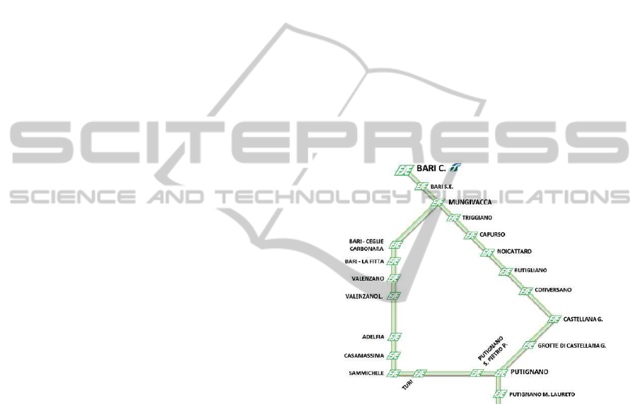
4 NUMERICAL EXPERIMENTS

The presented model is applied to Ferrovie del Sud

Est (FSE), the largest public transport company op-

erating in the Apulia region of Southern Italy. We

analyze the railway ring connecting Mungivacca and

Putignano stations (Figure 4), where a CTC system is

installed. The operation system is installed in Mun-

givacca station that is independent, not controlled by

the CTC, as is Putignano, whereby these stations are

not studied here. In particular, we refer to the line

1 of the railway ring – passing through Conversano

– that is single tracked except for the line connect-

ing Noicattaro to Rutigliano, that is double tracked.

Moreover, Grotte di Castellana is a single track sta-

tion, not chaired by an operator. 24 even trains and 22

odd trains run on the railway line during a day. We as-

sume a safety time ∆

= 3 min for two trains traveling

in opposite directions and a time ∆

= 1 min for trains

in the same direction. In attempt to evaluate the op-

timality of the algorithm, we used IBM CPLEX 12.5

installed and run on an Intel Core 2 Duo 1.83 GHz

CPU and 3 GB RAM, under Windows with the model

formulated in AMPL.

4.1 One Disturbance on the Line

We consider a real data set referring to a train going

from Putignano to Mungivacca that stops along the

line that connects Castellana G. and Conversano due

to a disturbance occurring at 7:50 am. That same dis-

turbance event is used for all the experiments but with

different disturbance sizes ∆

and solved with differ-

ent time horizons H. Various disturbance times are

been considered, ranging from 10 to 50 minutes. A

time horizon of H minutes means that movementsthat

should have started (according to the initial timetable)

H minutes or more after the instant at which the dis-

turbance occurs are not considered in the computa-

tion. Time horizons are expressed in minutes and

take values equal to 30, 60, 90, 120, 180, 240, 300,

360, 420, 480, 540, 600 and 1440. The main aspects

considered to present results are Obj

, Obj

Obj

that correspond respectively to sum of delays

for all train movements, delay of the last movement

of each train, number of rescheduled trains and num-

ber of rescheduled movements. All operational times

are given in minutes. CT refers to computational time

given in seconds. N and V refers to number of vari-

ables and constraints before and after the presolve

phase.

Figure 4: Ther railway ring used for the scenarios.

4.1.1 Overall Analysis

When only one disturbance occurs on the railway

line, results from experiments using the four objec-

tive functions for all different disturbance size (∆

)

and time horizons (H) are presented in Table 5.

The methodology is applied to a real case study in

which the occurence of short-term disturbance on the

railway line is frequent, this is not a trivial problem.

The model provides a proactive approach to solve, in

real time, problems that occur on the railway line.

The computational time (CT) for all time horizons

and disturbance sizes is of the order of a few sec-

ond. Comparison between different time horizons is

done in order to demonstrate that the model is able to

quickly solve even considerables problems that take

into account all trains on the railway line. In fact,

the highest value of CT (equal to 69.77 seconds) is

ICORES2014-InternationalConferenceonOperationsResearchandEnterpriseSystems

146

obtained using Ob j

for H = 1440 and ∆

= 45 min-

utes. This means that if a disturbance lasting 45 min-

utes occurs along the line, in just over a minute the

train dispatcher can obtain the rescheduled timetable

for the 24 hours following the occurrence of the fault.

The speed of resolution is a very important factor for

the presented problem, since the main objective of the

real-time trafﬁc management is to quickly establish

a new timetable, in order to minimize the inconve-

nience for passengers.

Compared to the previous methodology used in

(Dotoli et al., 2013) there is an improvement due to a

reduction of total delay, number of rescheduled trains

and computational time. The objective of this model

is the minimization of delay of all movements. In Ta-

ble 1 we compare results of the rescheduling process

obtained with the application of the actual and the

previous methodology (AM, PM) when ∆

= 30 min-

utes and H = 180 minutes. We noticed that Ob j

unchanged for all subsequent values of time horizon.

This means that the delay caused by the disturbance is

absorbed within the 180 minutes after its occurrence.

For the previous methodology, we present values ob-

tained for H = 30 minutes in addition to values ob-

tained with the application of the heuristic algorithm

after the time horizon. CT refers only at the optimiza-

tion procedure.

By analyzing values we observe that with the

actual methodology the new timetable is computed

in 0.72 seconds. Three trains are involved in the

rescheduling process for a total delay of 608 minutes.

Previous methodology required 10.74 seconds to ob-

tain the new timetable within a 30 minutes window

after the occurrence of the fault. 10 trains are involved

in the rescheduling process and total delay is equal to

665 minutes. Actual methodology allows to obtain

the optimal solution with an exact approach, with-

out the application of the heuristic algorithm which

does not always provide optimal results. We should

also take into account that solvers used by the two

methodology are different. MATLAB with GLPK

used by the previous methodologyis replaced by IBM

CPLEX in the actual one. Resolution methods used

by the two solvers are different as well as their per-

formance. The previous methodology has obtained an

improvement compared to the current practice used

by the train dispatcher; the actual methodology pro-

vides a further amelioration. This is in line with ob-

jectives of the real-time trafﬁc management.

4.1.2 Comparison between Objective Functions

We compare values obtained using the four objective

functions for H = 1440 and ∆

= 50 minutes, shown

in Table 2. We analyze the time horizon of 1440 min-

utes because the complexity of the problem is high

due to the presence, in the rescheduling process, of

all trains movements on the railway line until the end

of the day.

Lowest values in terms of total delay are obtained

using Obj

. Comparing results obtained with the ﬁrst

and the second objective function we notice that al-

though the value of Obj

is the same, Obj

changes.

In particular, Obj

obtained while Obj

is greater.

The reason is simple: in this case, minimizing the

delay of the last movement of a train, the second ob-

jective function increases the number of its delayed

movements. This means that although values of Obj

are unchanged using the ﬁrst and the second objec-

tive function, values of Obj

varies. In general, Obj

increases the arrival time at intermediate stations, in

order to minimize the delay at the last station of trains

path. In this case, there are no differences between

values of Obj

and Obj

obtained using Obj

and

Obj

. Extending the analysis to all time horizons, we

notice that in some cases (e.g. H = 180 and ∆

= 50

minutes) there is a difference between the two values,

due to the fact that these objective functions does not

take into account the exact dealy of trains. Thus, any

solution showing the same number of delayed trains is

optimal, whatever the value of Ob j

and Obj

. Mul-

ticriteria objective functions should be used to obtain

an unique optimal solution. The minimization of the

number of delayed trains (respectively movements)

may imply an increase of the total delay of resched-

uled trains.

Extending the analysis to values obtained in all

time horizons (H) and for all disturbance size (∆

) we

notice that minimizing Obj

provides better results in

terms of Ob j

and Ob j

. Minimizing Obj

provides

better values in terms of Obj

and Obj

4.1.3 Impact of Constraints (22), (23) and (24)

In order to prove the necessity of constraints (22),

(23) and (24) when using Ob j

and Obj

, we present

a simple railway line made by 7 segments on which

circulate 5 trains, represented in Figure 5. Railway

line is made by 4 single-tracked connection segment

and b

) between 3 double-tracked stations

, b

and b

). Trains t

and t

are directed to the

South, while t

, t

and t

travel in the opposite direc-

tion.

Table 1: Comparison between actual and previous method-

ology.

Obj

Our Methodology 608 3 0.72

Dotoli et al. 665 10 10.74

ARevisitedModelfortheRealTimeTrafficManagement

147

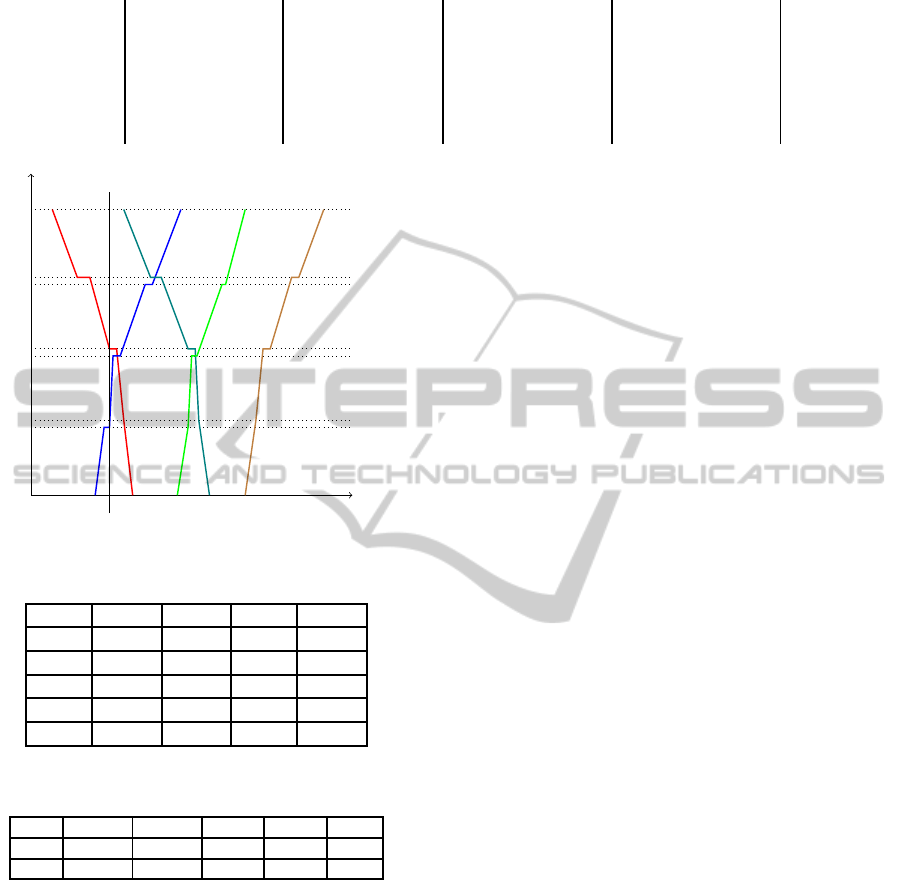
Table 4: Two independent disturbances.

FirstDisturbance SecondDisturbance TwoDisturbances Sum

Obj

516 61 1 9 13.43 308 61 3 26 17.98 824 122 4 35 31.41 824 122 4 36 17.95

Obj

516 61 1 9 11.95 308 61 3 26 17.63 824 122 4 35 29.58 826 122 4 36 19.83

Obj

516 61 1 9 9.08 336 71 1 5 9.81 852 132 2 14 18.89 871 132 2 14 9.16

Obj

516 61 1 9 10.42 336 71 1 5 12.21 852 132 2 14 22.63 871 132 2 14 10.12

= 07 : 35

time

Segment

Figure 5: Disturbance of t

Table 2: Comparison between the four objective functions

with H = 1440 and ∆

= 50.

Obj

829 854 878 878

Obj

81 81 91 91

Obj

3 3 1 1

Obj

33 39 11 11

CT 30.07 16.86 6.56 26.18

Table 3: Results from experiments using Obj

without and

with additional constraints.

Obj

WT 10040 10000 1 5 0.01

W 50 10 1 5 0.01

A disturbance occurs in the segment b

at 07:35

am and affects the train t

. We analyze a problem

with time horizon H = 25 minutes and a disturbance

size ∆

= 10 minutes. The same scenarios have been

solved without (WT) and with (W) the additional con-

straints using Obj

. Results are presented in Table 3.

By analyzing values of Ob j

and Obj

we notice

that despite the number of rescheduled trains is un-

changed, without the additional constraints the depar-

ture or the duration of some movements is delayed

for a long time. This means that minimizing Obj

tends to postpone movements of trains involved in the

rescheduling process at the end of the time horizon, in

order to affect the lowest number of trains on the line.

In the example, t

is the only delayed train. By in-

troducing additional constraints, values of Obj

(and

consequently Ob j

) are lower because the system is

forced to reschedule movements within the time hori-

zon. The number of rescheduled trains remains un-

changed.

4.2 Two Disturbances on the Line

When two independent disturbances occur on the rail-

way line, the rescheduling process of the ﬁrst distur-

bance does not inﬂuence the rescheduling process of

the second one. We consider the same railway line

presented in Section 4 and we suppose that two in-

dependent disturbances occur at T

= 09 : 00 a.m.

respectively in the line that connects Rutigliano to

Conversano stations (segment b

) and Conversano to

Castellana G. (segment b

). We consider a time hori-

zon H = 1440 minutes and a disturbance size ∆

= 50

minutes.

First, we solve the problem considering only the

disturbance that occurs in the segment b

and that af-

fects a train directed from Putignano to Mungivacca

station.

Then, we solve the problem considering only the

disturbance that occurs in the segment b

and that

affects a train directed from Mungivacca to Putignano

station.

Finally, we solve the problem considering the two

disturbances at the same time. We compare results

with those given by the sum of values obtained solv-

ing the two problems separately.

Table 4 presents values of Obj

, Ob j

, Obj

Obj

and CT for the four scenarios.

By comparing values obtained from simultaneous

resolution with those obtained from the sum of in-

dividual resolutions of disturbances, i.e. values pre-

sented in the third and the fourth block of Table 4,

we notice that the simultaneous resolution provides

a better result in terms of computational time for all

objective functions. However, the the sum of individ-

ual resolutions provides an improvement in terms of

Obj

and Ob j

using the four objective functions. In

particular by applying Obj

, there is a reduction of

the number of rescheduled movements and by apply-

ing Obj

, there is also a reduction of total delay. By

ICORES2014-InternationalConferenceonOperationsResearchandEnterpriseSystems

148

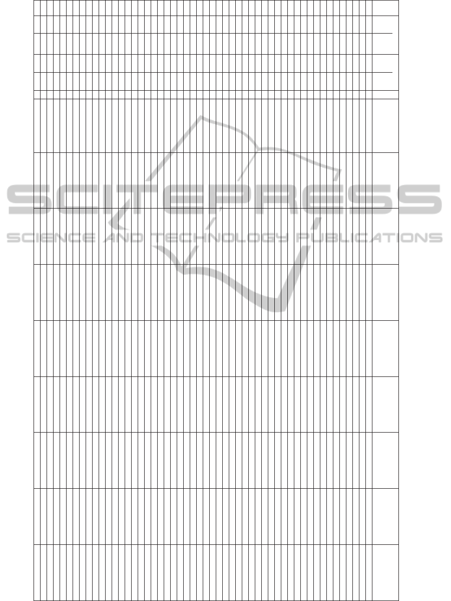
Table 5: Results of analysis using Obj

, Obj

and Obj

for all H and ∆

Tot. PrSlv ∆

= 10 ∆

= 15 ∆

= 20 ∆

= 25 ∆

= 30 ∆

= 35 ∆

= 40 ∆

= 45 ∆

= 50

Obj

30 6316 6555 1957 1897 1 70 10 1 7 0.04 105 15 1 7 0.04 140 20 1 7 0.03 175 25 1 7 0.06 210 30 1 7 0.03 245 35 1 7 0.04 280 40 1 7 0.03 315 45 1 7 0.03 350 50 1 7 0.10

30 6316 6555 1172 1897 2 70 10 1 7 0.05 105 15 1 7 0.05 140 20 1 10 0.08 175 25 1 10 0.01 210 30 1 10 0.05 245 35 1 10 0.03 280 40 1 10 0.16 315 45 1 10 0.03 350 50 1 10 0.06

30 6316 7047 1960 1897 3 70 10 1 7 0.14 105 15 1 7 0.47 140 20 1 7 0.05 175 25 1 7 0.05 210 30 1 7 0.03 245 35 1 7 0.05 280 40 1 7 0.05 315 45 1 7 0.05 350 50 1 7 0.05

30 6472 7359 1972 1921 4 70 10 1 7 0.06 105 15 1 7 0.03 140 20 1 7 0.05 175 25 1 7 0.03 210 30 1 7 0.05 245 35 1 7 0.05 280 40 1 7 0.03 315 45 1 7 0.05 350 50 1 7 0.20

60 7636 8190 2675 2818 1 110 10 1 11 0.07 211 23 3 25 0.09 296 31 2 19 0.09 367 36 2 21 0.09 428 43 2 13 0.08 433 43 2 13 0.07 450 45 2 13 0.09 515 55 2 13 0.06 580 65 2 13 0.06

60 7636 8190 2675 2818 2 110 10 1 11 0.06 211 23 3 19 0.08 300 31 2 21 0.09 367 38 3 21 0.12 428 43 2 21 0.18 437 43 2 23 0.09 450 45 2 23 0.09 470 55 2 26 0.09 610 56 1 26 0.08

60 7636 8758 2678 2814 3 110 10 1 11 0.06 304 38 2 19 0.09 300 31 2 19 0.08 531 61 2 13 0.08 667 75 2 19 0.08 595 56 1 11 0.06 600 56 1 11 0.06 605 56 1 11 0.08 610 56 1 11 0.09

60 7816 9118 2690 2831 4 110 10 1 11 0.07 304 38 2 19 0.12 502 69 2 13 0.09 567 79 2 13 0.08 428 43 2 13 0.11 595 56 1 11 0.08 600 56 1 11 0.08 605 56 1 11 0.09 610 56 1 11 0.08

90 8920 10074 3401 3995 1 110 10 1 11 0.12 266 31 2 21 0.30 310 31 2 21 0.20 431 44 6 44 0.23 512 51 5 34 0.21 517 55 5 34 0.20 554 58 4 32 0.30 697 76 3 28 0.28 751 69 1 11 0.45

90 8920 10074 3401 3995 2 110 10 1 11 0.12 289 31 2 21 0.12 310 31 2 23 0.05 431 44 6 23 0.90 540 55 4 23 0.20 517 55 5 34 0.16 572 58 5 34 0.22 752 69 1 35 0.23 751 69 1 35 0.20

90 8920 10712 3380 3937 3 110 10 1 11 0.06 913 83 1 11 0.17 891 83 1 11 0.18 913 83 1 11 0.18 891 83 1 11 0.18 892 83 1 11 0.17 913 83 1 11 0.12 878 83 1 11 0.18 913 83 1 11 0.20

90 9122 11916 3436 4848 4 110 10 1 11 0.08 913 83 1 11 0.20 891 83 1 11 0.22 913 83 1 11 0.20 913 83 1 11 0.23 892 83 1 11 0.22 891 83 1 11 0.22 751 69 1 11 0.18 913 83 1 11 0.23

120 10519 12275 4345 5762 1 110 10 1 11 0.20 266 31 2 21 0.42 310 31 2 21 0.28 477 46 7 67 0.51 586 68 5 39 0.36 591 68 5 39 0.36 616 69 5 39 0.56 753 82 5 45 0.73 814 80 2 18 0.88

120 10519 12275 4345 5762 2 110 10 1 11 0.17 289 31 2 21 0.50 310 31 2 23 0.37 477 46 7 23 0.40 604 59 6 23 0.45 609 59 6 35 0.40 672 65 6 35 0.55 839 80 2 36 1.18 838 80 2 39 0.62

120 10519 12996 4192 5290 3 110 10 1 11 0.14 864 82 2 18 0.45 406 47 2 18 0.40 864 82 2 18 0.40 857 82 2 18 0.40 864 83 2 18 0.28 847 80 2 18 0.28 878 82 2 18 0.30 830 81 2 18 0.26

120 10748 13454 4279 5467 4 110 10 1 11 0.18 855 82 2 18 0.44 864 83 2 18 0.72 856 82 2 18 0.50 833 80 2 18 0.50 863 82 2 18 0.36 861 82 2 18 0.33 863 82 2 18 0.30 830 81 2 18 0.31

180 13051 16644 5925 9048 1 110 10 1 11 0.3 266 31 2 21 0.95 310 31 2 21 0.50 523 48 8 90 0.83 608 76 3 29 0.72 613 76 3 29 0.62 638 77 3 29 1.17 829 81 3 33 0.51 829 81 3 33 1.40

180 13051 16644 5925 9048 2 110 10 1 11 0.31 267 31 2 21 1.12 310 31 2 23 0.60 523 48 8 23 0.73 714 65 8 23 0.68 719 65 8 35 0.80 825 73 8 35 1.30 853 81 3 36 1.68 853 81 3 39 0.99

180 13051 17485 5916 9008 3 110 10 1 11 0.17 875 91 1 11 0.64 875 91 1 11 0.65 875 91 1 11 0.64 875 91 1 11 0.61 875 91 1 11 0.61 875 91 1 11 0.67 875 91 1 11 0.64 948 91 1 11 0.48

180 13318 18019 6037 9249 4 110 10 1 11 0.20 875 91 1 11 0.70 875 91 1 11 0.72 875 91 1 11 0.75 875 91 1 11 0.81 875 91 1 11 0.69 875 91 1 11 0.80 875 91 1 11 0.75 875 91 1 11 0.72

240 18149 21612 7721 13225 1 110 10 1 11 0.31 266 31 2 21 3.01 310 31 2 21 0.98 523 48 8 90 1.87 608 76 3 29 1.99 613 76 3 29 1.64 638 77 3 29 2.20 829 81 3 33 8.16 829 81 3 33 8.35

240 15804 43004 5376 24173 2 110 10 1 11 0.30 267 31 2 21 2.24 314 31 2 23 1.46 523 48 8 23 1.31 716 65 8 23 1.56 721 65 8 35 1.50 820 73 8 35 2.11 855 81 3 36 2.84 853 81 3 39 1.98

240 15804 22574 7684 13117 3 110 10 1 11 0.31 875 91 1 11 0.70 875 91 1 11 0.78 875 91 1 11 0.15 875 91 1 11 0.84 875 91 1 11 0.78 875 91 1 11 0.90 875 91 1 11 0.81 875 91 1 11 0.96

240 16110 23186 7844 13436 4 110 10 1 11 0.36 875 91 1 11 0.95 875 91 1 11 0.90 875 91 1 11 0.95 875 91 1 11 0.90 875 91 1 11 1.01 875 91 1 11 0.99 875 91 1 11 0.90 875 91 1 11 1.01

300 17528 25234 8889 16141 1 110 10 1 11 0.57 266 31 2 21 3.91 310 31 2 21 2.31 523 48 8 90 2.88 608 76 3 29 2.77 613 76 3 29 2.56 638 77 3 29 2.96 829 81 3 33 7.05 829 81 3 33 5.04

300 17528 25234 8889 16141 2 110 10 1 11 0.37 289 31 2 21 2.04 318 31 2 26 1.23 523 48 8 23 1.90 716 65 8 23 2.42 721 65 8 35 1.95 820 73 8 35 2.43 854 81 3 36 3.62 853 81 3 39 2.01

300 17528 26266 8892 16115 3 110 10 1 11 0.40 875 91 1 11 1.01 875 91 1 11 0.89 875 91 1 11 0.98 875 91 1 11 0.94 875 91 1 11 1.01 875 91 1 11 1.07 875 91 1 11 0.93 875 91 1 11 1.06

300 17856 26922 9074 16478 4 110 10 1 11 0.44 875 91 1 11 1.25 875 91 1 11 1.17 875 91 1 11 1.20 875 91 1 11 1.34 875 91 1 11 1.25 875 91 1 11 1.23 875 91 1 11 1.12 875 91 1 11 1.22

360 20240 30791 10762 20933 1 110 10 1 11 0.78 266 31 2 21 3.04 310 31 2 21 1.77 523 48 8 90 3.44 608 76 3 29 3.33 613 76 3 29 2.85 638 77 3 29 4.29 829 81 3 33 12.48 829 81 3 33 5.55

360 20240 30791 10762 20933 2 110 10 1 11 0.51 319 31 2 21 3.20 324 31 2 23 2.07 523 48 8 23 2.48 716 65 8 23 2.92 721 65 8 35 2.84 820 73 8 36 4.47 855 81 3 36 4.37 854 81 3 39 4.70

360 20240 31929 10575 20491 3 110 10 1 11 0.87 875 91 1 11 1.34 875 91 1 11 1.22 875 91 1 11 1.30 875 91 1 11 1.18 875 91 1 11 1.38 875 91 1 11 1.26 875 91 1 11 1.34 875 91 1 11 1.32

360 20602 32653 10791 20922 4 110 10 1 11 1.12 875 91 1 11 1.48 875 91 1 11 1.57 875 91 1 11 1.51 875 91 1 11 1.48 875 91 1 11 1.64 875 91 1 11 1.46 875 91 1 11 1.40 875 91 1 11 1.64

420 23226 37541 12889 26619 1 110 10 1 11 0.98 266 31 2 21 3.52 310 31 2 21 2.29 523 48 8 90 5.66 608 76 3 29 4.76 613 76 3 29 3.66 638 77 3 29 6.50 829 81 3 33 19.40 829 81 3 33 10.28

420 23226 37541 12889 26619 2 110 10 1 11 0.68 289 31 2 21 3.80 314 31 2 23 3.20 523 48 8 23 3.43 716 65 2 23 3.57 721 65 8 35 3.40 840 73 8 35 5.27 853 81 3 36 6.32 853 81 3 39 4.15

420 23226 38787 12892 26585 3 110 10 1 11 0.69 875 91 1 11 1.73 875 91 1 11 1.62 875 91 1 11 1.68 875 91 1 11 1.64 875 91 1 11 1.73 875 91 1 11 1.80 875 91 1 11 1.65 875 91 1 11 1.81

420 23622 39579 13142 27084 4 110 10 1 11 0.76 875 91 1 11 2.03 875 91 1 11 2.06 875 91 1 11 2.07 875 91 1 11 2.12 875 91 1 11 2.07 875 91 1 11 1.60 875 91 1 11 1.88 875 91 1 11 2.12

480 26152 44235 14868 32237 1 110 10 1 11 1.74 266 31 2 21 5.52 310 31 2 21 2.71 523 48 8 90 5.21 608 76 3 29 4.66 613 76 3 29 4.62 638 77 3 29 8.70 829 81 3 33 31.04 829 81 3 33 9.70

480 26152 44235 14868 32237 2 110 10 1 11 1.36 267 31 2 21 5.63 324 31 2 23 4.08 523 48 8 23 4.93 716 65 8 23 4.85 721 65 8 35 4.77 820 73 8 35 7.63 853 81 3 36 8.05 853 81 3 39 6.47

480 26152 45601 14729 31903 3 110 10 1 11 1.35 876 91 1 11 2.54 876 91 1 11 2.21 876 91 1 11 2.18 876 91 1 11 2.18 876 91 1 11 2.14 876 91 1 11 2.18 876 91 1 11 2.26 876 91 1 11 2.21

480 26586 46469 15017 32478 4 110 10 1 11 1.57 876 91 1 11 2.40 876 91 1 11 2.37 876 91 1 11 2.43 876 91 1 11 2.37 876 91 1 11 2.40 876 91 1 11 2.30 876 91 1 11 2.42 876 91 1 11 2.42

540 29808 53122 17727 40361 1 110 10 1 11 1.66 266 31 2 21 12.53 310 31 2 21 4.30 523 48 8 90 7.72 608 76 3 29 6.75 613 76 3 29 8.83 638 77 3 29 12.96 829 81 3 33 30.15 829 81 3 33 18.48

540 29808 53122 17727 40361 2 110 10 1 11 1.72 267 31 2 21 7.58 314 31 2 24 5.55 523 48 8 24 2.14 716 65 8 24 5.60 721 65 8 36 6.16 820 73 8 36 9.36 853 81 3 36 10.98 853 81 3 39 7.59

540 29808 54588 17314 39441 3 110 10 1 11 1.74 875 91 1 11 2.71 875 91 1 11 2.80 875 91 1 11 2.73 875 91 1 11 2.93 875 91 1 11 2.70 875 91 1 11 2.79 875 91 1 11 3.85 875 91 1 11 2.87

540 30274 55520 17634 40080 4 110 10 1 11 1.87 875 91 1 11 2.87 875 91 1 11 2.99 875 91 1 11 2.92 875 91 1 11 3.00 875 91 1 11 2.94 875 91 1 11 3.32 875 91 1 11 3.07 875 91 1 11 3.20

600 33335 61819 20398 48293 1 110 10 1 11 2.07 266 31 2 21 12.87 310 31 2 21 4.60 523 48 8 90 10.12 608 76 3 29 8.52 613 76 3 29 8.13 638 77 3 29 10.15 829 81 3 33 38.12 829 81 3 33 15.33

600 33335 61819 20398 48293 2 110 10 1 11 2.15 267 31 2 21 8.92 321 31 2 24 7.84 523 48 8 24 6.86 716 65 8 24 6.58 721 65 8 36 7.06 834 73 8 36 10.75 867 81 3 36 12.45 853 81 3 39 9.41

600 33335 63394 20131 47675 3 110 10 1 11 2.23 877 91 1 11 3.26 877 91 1 11 3.66 878 91 1 11 3.54 877 91 1 11 3.43 877 91 1 11 3.60 877 91 1 11 3.45 877 91 1 11 3.54 877 91 1 11 3.62

600 33836 64396 20486 48384 4 110 10 1 11 2.12 877 91 1 11 3.46 877 91 1 11 3.54 878 91 1 11 3.66 877 91 1 11 3.60 877 91 1 11 3.62 877 91 1 11 3.70 877 91 1 11 3.52 877 91 1 11 3.73

1440 48247 101160 32059 84305 1 110 10 1 11 3.85 266 31 2 21 22.40 310 31 2 21 9.17 523 48 8 90 19.81 608 76 3 29 17.08 613 76 3 29 16.55 638 77 3 29 20.23 829 81 3 33 69.77 829 81 3 33 30.07

1440 48247 101160 32059 84305 2 110 10 1 11 3.96 266 31 2 21 21.60 332 31 2 23 17.94 523 48 8 24 14.43 716 65 8 24 14.24 721 65 8 36 14.22 820 73 8 34 22.37 853 81 3 36 24.27 854 81 3 39 16.86

1440 48247 103146 31766 83615 3 110 10 1 11 4.40 878 91 1 11 6.60 878 91 1 11 7.08 878 91 1 11 6.32 878 91 1 11 6.58 878 91 1 11 6.97 878 91 1 11 6.95 878 91 1 11 8.47 878 91 1 11 6.56

1440 48879 104428 32252 84586 4 110 10 1 11 2.99 878 91 1 11 5.63 878 91 1 11 5.27 878 91 1 11 6.64 878 91 1 11 9.64 878 91 1 11 14.21 878 91 1 11 14.28 878 91 1 11 11.23 878 91 1 11 26.18

ARevisitedModelfortheRealTimeTrafficManagement

149

using Obj

and Obj

, there is a decrease of values

of Obj

. However, it is interesting to note that when

multiple independent disturbances occur on the line,

it is possible to decompose the problem in indepen-

dent subproblems. In this way, the train dispatcher

can give priority to the rescheduling of trains which

paths include stations where a higher level of service

is required or that have to comply connections with

other trains. One could expect that two disturbances

would be more difﬁcult to solve but, according to the

ﬁrst experiments, this is not the case. More particu-

larly, the time needed to solve the ﬁrst disturbance is

greater than the time needed to solve both, perhaps

due to number of embedded variables. More explicit,

we are in progress to verify that.

5 CONCLUSIONS AND

PERSPECTIVES

In this paper, we propose a formalization of the

rescheduling real-time problem for a regional single-

tracked railway network in which a CTC control sys-

tem is installed. We propose a mathematical model

that operates as a decision support system for the train

dispatcher. The main goal is to ﬁnd a decision support

system for the train dispatcher that is able to restore

normal trafﬁc conditions after the occurrence of a dis-

turbance and to provide an adequate level of service

to passengers. We analyze four alternative objective

functions in order to ﬁnd the optimal solution that is

a good compromise between total delay, number of

rescheduled trains and computational time.

There are many perspectives for this work:

- increase the complexity of the analysis, consider-

ing a greater number of disturbances on the line

that occur at different times and have different

size.

- introduce robustness in the rescheduling process.

A robust rescheduled timetable is less subject to

change if a new disturbance occurs on the railway

line.

- perform a structural analysis of the railway line

in order to verify if there are independent sectors

in which it is possible to predetermine an optimal

solution to applied when a disturbance occours.

- introduceindicators of the complexity of the prob-

lem in order to assess the sensibility of the com-

putational time with these parameters.

- include a resolution strategy that allow the cancel-

lation of a train when the delay that it would accu-

mulate along the line exceeds a certain threshold.

- study other resolution methods most suitable to

the complexity of the problem, such as constraints

programming, able toproduce a setof possible so-

lutions.

REFERENCES

D’Ariano, A. (2008). Real-Time Train Dispatching: Mod-

els, Algorithms and Applications. PhD thesis, Fac-

ulty of Civil Engineering and Geosciences, Delft Uni-

versity of Technology, Department of Transport and

Planning.

Dotoli, M., Epicoco, N., Falagario, M., Piconese, A., Scian-

calepore, F., and Turchiano, B. (2013). A real time

trafﬁc management model for regional railway net-

works under disturbances. In 9th annual IEEE Confer-

ence on Automation Science and Engineering , Madi-

son, USA.

FSE - Ferrovie del Sud Est (2013). Fse - ferrovie del sud est

e servizi automobilistici. http://www.fseonline.it.

Ismail, S. (1999). Railway trafﬁc control and train schedul-

ing based on inter-train conﬂict management. Trans-

ports Research, Part B, 33:511–534.

Vicuna, G. (1989). Organizzazione e tencica ferroviaria.

Vol. II. CIFI; Collegio Ingegneri Ferroviari Italiani,

Roma.

ICORES2014-InternationalConferenceonOperationsResearchandEnterpriseSystems

150