Geographic Routing with Partial Position Information

∗

Tony Ducrocq

, Micha

el Hauspie

and Nathalie Mitton

Inria Lille - Nord Europe, 59650 Villeneuve d’Ascq, France

Universit

e Lille1, Cit

e Scientiﬁque, 59100 Lille, France

Keywords:

Wireless Sensor Networks, Geographic Routing Algorithm, Position Based Routing.

Abstract:

Geographic routing protocols show good properties for Wireless Sensor Networks (WSN). They are stateless,

local and scalable. However they require that each node of the network is aware of its own position. While it

may be possible to equip each node with GPS receiver, even if it is costly, there are some issues and receiving

a usable GPS signal may be difﬁcult in some situations. For these reasons, we propose a geographic routing

algorithm, called

HGA

, able to take advantages of position informations of nodes when available but also

able to continue the routing in a more traditional way if position information is not available. We show with

simulations that our algorithm offers an alternative solution to classical routing algorithm (non-geographic) and

offers better performances for network with a density above

and more than

of nodes are aware of their

position.

1 INTRODUCTION

Wireless sensor networks consist of sets of mobile

wireless nodes without the support of any ﬁxed infras-

tructure. Such wireless sensor networks offer great

application perspectives. Sensors are tiny devices with

hardware constraints (low memory storage, low com-

putational resources) that rely on battery. Sensor net-

works thus require energy-efﬁcient algorithms to make

them work properly in a way that suits their hardware

features and application requirements.

Low power sensor nodes have limited transmission

power, thus they can communicate only to a limited

number of nodes. This set of nodes is called the neigh-

borhood of the node. In order to send messages at

longer range, nodes are using multi-hop communica-

tion. Multi-hop communication means that data will

need to be routed from source to destination by other

nodes. An efﬁcient way to route messages is to use

nodes position information. A node uses a metric

based on its own position, its neighbors positions and

the destination position in order to choose the next hop

for the route. To use such a technique it is possible to

equip each node of the network with a GPS receiver or

to conﬁgure them at setup with their position if they

are static.

∗

This work is partially supported by CPER Nord-Pas-

de-Calais/FEDER Campus Intelligence Ambiante and ANR

ECOTECH BinThatThinks.

On the other hand there exist non geographic rout-

ing algorithms. They do not require node position to

route data but only neighborhood knowledge.

In the Smart Cities context, it is likely that the net-

work is heterogeneous (Al-Hader et al., 2009). Some

nodes may be aware of their position while some other

are not. The reason to not equip nodes with GPS re-

ceiver may be to save money or energy. It is also not

possible to setup position of mobile nodes as it will

change over time. Furthermore, even if all nodes are

equipped with a GPS receiver, it is possible that some

of them do not receive the signal because of environ-

mental factors. For instance, two districts of a city may

be connected through a tunnel, in which GPS signal is

not received.

In such contexts, the availability of a routing al-

gorithm taking advantages of nodes positions when

possible but also functioning when the position is

not available is interesting. Thus, we introduce the

HGA

algorithm (

ybrid-

reedy-

ODV). The algo-

rithm works like the Greedy geographic routing while

position information allows it, and if position informa-

tion is not available, a route request message is sent in

the node neighborhood in order to ﬁnd a path toward

the destination.

The rest of the paper is organized as follows: Sec-

tion 2 presents related work concerning geographic

and pseudo geographic routing algorithms. We intro-

duce some background works on which our algorithm

165

Ducrocq T., Hauspie M. and Mitton N..

Geographic Routing with Partial Position Information.

DOI: 10.5220/0004872901650172

In Proceedings of the 3rd International Conference on Sensor Networks (SENSORNETS-2014), pages 165-172

ISBN: 978-989-758-001-7

 2014 SCITEPRESS (Science and Technology Publications, Lda.)

relies in Section 3. Section 4 describes the

HGA

algo-

rithm operation in details and Section 5 present sim-

ulation and results of its performances. Finally we

conclude in Section 6.

2 RELATED WORKS

To the best of our knowledge, there is no existing rout-

ing solution that considers that only a subset of nodes

is aware of its position. Classical routing algorithms

and those using virtual coordinates are the closest ap-

proaches to the one we propose. In this section we

describe related works as well as works on which our

proposal relies.

The main idea of geographic routing protocols is to

route data closer to the destination at each step of the

routing. The Greedy algorithm, on which part of our

work relies, chooses the closest node to the destination

in a node’s neighborhood as the next forwarder of the

data packet. The Greedy algorithm and some variants

from literature are shown on Figure 1.

Figure 1: Comparison of geographic algorithms. Node

is chosen by MFR algorithm, node

by Greedy, node

NFP and node e by Compass.

Some algorithms allow the deduction of position

for nodes by using their neighbors (

Capkun et al.,

2002), (Ermel et al., 2005). Nevertheless, these so-

lutions exhibit poor performances due to the difﬁculty

to determine distance between two nodes without spe-

cialized hardware (Benkic et al., 2008). Moreover,

Seada et al. (Seada et al., 2004) showed that a small

error on position can generate several losses of packets

in geographic routing algorithms.

Routing algorithms over virtual coordinates allow

the beneﬁts of geographic routing algorithms without

the need of real geographic position of nodes. The

main drawback of these solutions resides in the setup

of the virtual coordinates system. Indeed, it is needed

to ﬂood all the network several times at the beginning

of the network lifetime.

The VCap solution (Caruso et al., 2005) relies on

virtual coordinates and a greedy routing. Some partic-

ular nodes are chosen for their interesting properties

to act as starting points for the different coordinates

of the system. These nodes are named anchors. The

coordinate system relies on the distance in number

of hops between a node and the different anchors. A

predeﬁned sink node is used to initiate anchors elec-

tion (or any other node). This node, by broadcasting

a message in the whole network allows to elect a ﬁrst

anchor. At its turn, this anchor broadcast a message

in the whole network to elect a second one and so on.

Anchors are chosen to be close to the network bound-

aries a far away to each other to limit duplicates in

coordinates. In VCap the network is ﬂooded at least

times. Otherwise, because uniqueness of coordinates

is not guaranteed, the delivery can not be guaranteed.

The cost over progress concept idea (Stojmenovic,

2006) is to optimize the ratio between the cost of a

transmission by the progress made by the transmission.

Vcost (Elhafsi et al., 2007) relies on this idea and on

VCap coordinate system to reduce energy needs for

the routing.

The LTP algorithm (Ch

avez et al., 2007) uses a

root and a tree construction as the only coordinate

system instead of anchors. Thanks to the tree, this

routing algorithm guarantees delivery but the chosen

routes may be long. Above all, the tree construction is

costly and hard to maintain.

HECTOR (Mitton et al., 2012) combines both co-

ordinates systems of LTP and VCap. Its chooses the

best node in the VCap coordinate system at the same

level or that allow a progress in LTP coordinate system.

HECTOR is then able to guarantee delivery of packets

and to reduce the energy used for the routing.

Other virtual coordinates solutions have been pro-

posed, some are without guaranteed delivery (Ben-

badis et al., 2006), (Fang et al., 2005), (Niculescu

and Nath, 2001), some other with guaranteed deliv-

ery (Ch

avez et al., 2007), (Liu and Abu-Ghazaleh,

2008). However, algorithms using virtual coordinates

have the drawback to not support node mobility. Fur-

thermore, it is needed to ﬂood the whole network at the

beginning, introducing high latency at startup when

the network is big.

3 BACKGROUND

Our proposal relies on route requests and route replies

similar to those used in AODV (Perkins and Royer,

1999). We introduce their behavior in the following.

Figure 2 shows a route search in AODV.

AODV is a non-geographic routing, totally reactive.

SENSORNETS2014-InternationalConferenceonSensorNetworks

166

(a) Reverse path setup.

(b) Forward path setup.

Figure 2: Route search example from S to D in AODV.

Indeed, routes are established only on-demand, when

they are needed. To route a data packet toward the

destination, a node broadcasts a RREQ (route request)

in its neighborhood. Each node receiving the RREQ

keeps track of it until expiration delay expires (deﬁned

3000 ms

in AODV). Keeping track of RREQ allows

the creation of the reverse path as shown in Figure 2(a)

that will be used when destination is found. If a node

S does not know a route towards the destination D,

S is not the destination and it has not received this

RREQ earlier, it broadcasts a RREQ at its turn in its

neighborhood. When a node knows a route toward

the destination, or is itself the destination, it sends a

RREP packet (route reply) to the node that has sent

the RREQ. The RREP packet then follows the reverse

path and each node on the route saves the source of

the RREP in its neighborhood table in order to create

the reverse path. Figure 2(b) shows the creation of the

forward path and expiration of reverse paths.

4 PROPOSAL

In this paper, we propose

HGA

, a

ybrid

reedy-

ODV algorithm. The main idea of

HGA

is to apply

a greedy geographic routing whenever it is possible.

When a greedy routing is not possible, a RREQ is sent

in the

-neighborhood of the node. When a node needs

to route a data packet and none of its neighbors allows

a progress toward the destination, a route is searched

in AODV fashion (Perkins and Royer, 1999).

We ﬁrst describe the notations and the model used

and then the algorithm details.

4.1 Notations and Model

The

parameter is the maximum depth for searching

a route and deﬁnes the variant of HGA : HGA-

. The

set of nodes aware of their position is

, then if

knows its position

u ∈ P

deﬁnes the routing table

of a node, then

R(u)

is the routing table of node

RREQ T IMEOU T

is the delay until a RREQ is ig-

nored if no RREP has been received. The Euclidean

distance between nodes

and

is noted

|uv|

N(u)

is the set of neighbors in communication range of

RREQs in the “waiting” state belong to the set W .

4.2 Algorithm Description

The header of a data packet contains the destination

position and the last known position where the packet

passed by.

To route a data packet, a node

starts by verifying

if one of its neighbors allows a progress toward the

destination. If

knows its own position, the progress

depends of the distance between

and the destina-

tion. If

is not aware of its position, the progress

depends on the last known position contained in the

data packet if available, otherwise, any node aware of

its position will be considered as making a progress.

If no neighbor of

allows a progress,

R(u)

is sought

to ﬁnd a route allowing a progress in an AODV fash-

ion. If there is no such a route, a RREQ is sent

N(u)

and a new research in routing table is made after the

delay

RREQ T IMEOU T

. Algorithm 1 sums up route

search on a node u.

When u receives a RREQ, it can either transmit it,

answer with a RREP or discard it. Node

starts by

analyzing

R(u)

to verify, by comparing the sequence

number and the source node of RREQ to those in the

routing table entries, whether

has already received

this RREQ. If so, the RREQ is ignored and nothing

happens, otherwise

search in

N(u)

if a node is closer

to the destination than the source of the RREQ. If a

route is found among neighbors of

, a RREP is sent

to the nodes that transmitted the RREQ to

. The

RREP contains the source id and sequence number

from the RREQ, it also contains position of the closest

neighbor of

to destination. If no route is found, the

RREQ is forwarded if the maximum depth

for RREQ

(

MAX HOP RREQ

) has not been reached. When a

RREQ is transmitted, a new entry in the routing table

is created with a ‘waiting” ﬂag allowing to know that a

RREQ has been sent but no route is known yet. Algo-

rithm 2 describes operations made at RREQ reception.

When a RREQ is received by a node

, the corre-

sponding entry with “waiting” ﬂag in the routing table

is updated. The ﬂag is removed and the neighbor allow-

ing the destination to be reached is written is the table

(this information is known thanks to the RREQ). Like-

wise, position of the destination is updated, indeed, the

RREP may point to a position allowing to approach

the destination but not necessarily the destination itself.

By saving position of the node contained in the RREQ,

routing table informations are more accurate.

GeographicRoutingwithPartialPositionInformation

167

Algorithm 1:

Data packet reception at node

towards

with

being last node with known

position.

1 if u = D then

2 exit /* success */ ;

3 next ← −1 ;

4 if u ∈ P then

5 dist ← |uD| ;

6 l ← u ;

7 else if l 6= −1 then

8 dist ← |lD| ;

9 else

10 dist ← +∞ ;

11 for v ∈ N(u) do

12 if |vD| < dist then

13 next ← v ;

14 dist ← |vD| ;

15 if next < 0 then

16 /* no route found in direct neighborhood */

17 broadcast(RREQ) ;

18 R ← R ∪ RREQ ;

19 W ← W ∪RREQ ;

20 wait(RREQ TIMEOUT) ;

21 if ¬(∃r,r ∈ R ∧ |rD| < dist) ∧ r /∈ W then

22 R ← R \ RREQ ;

23 /* no route found */

24 drop(data) ;

25 exit /* fail */ ;

26 else

27 for r ∈ R do

28 /* For each known route */

29 if |rD| < dist then

30 dist ← |rD| ;

31 next ← r ;

32 send(data, next) /* data transmitted */ ;

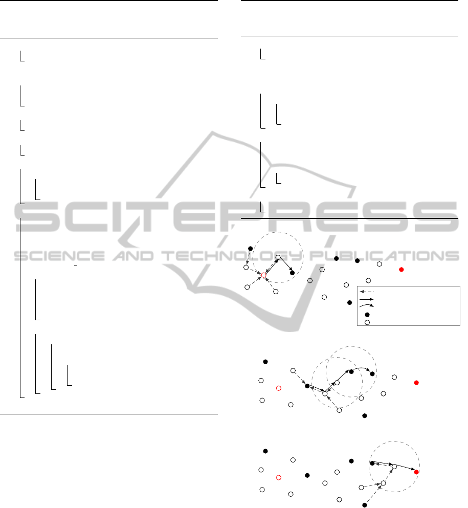
HGA does not guarantee delivery, indeed if no

node in the

-neighborhood of a node is aware of its

position, the node will not be able to route packets.

However, the route search mechanism allows to cir-

cumvent dead ends by searching new routes in the

-hops limit. Figure 3 shows an example of routing

from node

, which is not aware of its position, to

aware of its position. Figure 3(a) highlights a route

request with a maximum depth of

. Nodes receiving

the RREQ and knowing their position answer with a

RREP and

chooses the one which allow the max-

imum progression to destination. Once the packet

has been routed to the intermediate destination, a new

RREQ is initiated, the packet continues its progression

then it is routed using classical geographic routing

technique as intermediate destination knows a neigh-

bor allowing a progression through destination 3(b).

Finally, on Figure 3(c) a last RREQ is performed to

Algorithm 2:

Reception of a RREQ initiated by

with sequence number

seqnum

on node

for

destination D.

1 if (S,seqnum) ∈ R then

2 exit /* RREQ already sent */;

3 next ←

0 ;

4 dist ← |SD| ;

5 for v ∈ N(u) do

6 if |vD| < dist then

7 next ← v ;

8 dist ← |vD| ;

9 if next =

0 then

10 hop ← hop − 1 ;

11 R ← R ∪ RREQ ;

12 if hop > 0 then

13 broadcast(RREQ) ;

14 else

15 send(RREP, u,next) ;

Reverse path

Forward path

Geographic routing

Node with position

Node without position

(a) First RREQ.

(b) Second RREQ and geograhic routing.

Figure 3: Routing example in HGA.

allow the destination to be reached.

5 SIMULATION AND RESULTS

We choose to compare HGA to VCap, a routing algo-

rithm using a similar greedy routing technique but

SENSORNETS2014-InternationalConferenceonSensorNetworks

168

based on virtual coordinates. We also simulate a

greedy routing algorithm, slightly adapted to operate

with some nodes without position awareness. In this

variant, nodes without position knowledge do not send

HELLO messages, then they do not participate in rout-

ing but can emit data packets. When a node needs to

send a data packet (because it is the source or it needs

to transfer it), it chooses in its neighbors with position

the closest to the destination allowing a progress. If

the node sending the data packet is not aware of its

position, the notion a progress does not exist, then

the closest position aware neighbor to destination is

chosen.

We simulated HGA with route search depth of

and

hops. VCap has been simulated with

and

5 anchors.

Simulations have been performed using WS-

NET (Fraboulet et al., 2007) simulator. Each sim-

ulation lasts for

minutes. We generated random

connected topologies of

500

750

1000

1500

2000

2500

and

3000

nodes in a ﬁeld of

500 m × 500 m

achieve average density of

nodes per communication range. Nodes have a com-

munication range of

40 m

. Each combination (algo-

rithm, average density) is launch

times on different

topologies. The same topology is used for a combina-

tion of average density and iteration number for each

different algorithm. For instance the ﬁrst simulation

of HGA-1 uses the same topology as the simulation of

VCap-3, Greedy, etc.

To simulate a data trafﬁc, every

seconds, each

node chooses randomly a destination node aware of

its position. The source node sends the data packet in

respect to the algorithm it executes. Nodes are desyn-

chronized in order to distribute emissions in time.

We measure delivery ratio, control message num-

ber and memory used. The delivery ratio is the number

of messages received divided by the number of mes-

sages sent. Control messages are HELLO, RREQ,

RREP and messages to initiate the coordinate sys-

tem. Finally, the memory used is the average num-

ber of neighbors saved by a node plus the number of

known routes for each node. Simulation parameters

are summed up in Table 1.

For the sake of clarity, in the following we refer to

HGA with a depth search of

hop by HGA-

(

k = 1

Moreover, HGA-

(resp. HGA-

and HGA-

) refer to

HGA algorithm with depth search of

(resp

and

)

hops. Finally VCap-

and VCap-

refer to the VCap

algorithm with

and

anchors. VCap results curves

have been duplicated on ﬁgures with

and

10%

located nodes in order to ease readings.

Table 1: Simulation parameters.

Parameter Value

Duration (m) 10

MAC layer idealmac

Interferences none

Data size (bytes) 10

Header size (bytes) 88

Field size 500 m× 500 m

Communication range 40 m

Number of nodes 500, 750, 1000, 1500, 2000, 2500, 3000

Density 10, 15, 20, 30, 40, 50, 60

Iterations 50

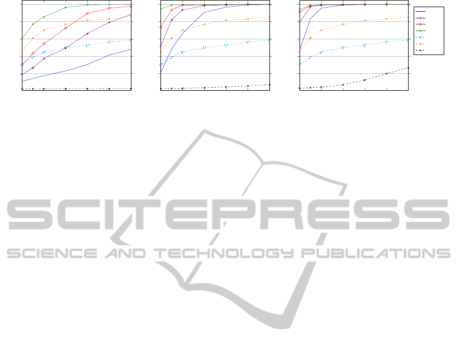
5.1 Delivery Ratio

Figure 4 shows delivery ratio for the four variants

of HGA, the two variants of VCap and the Greedy

algorithm. We can see on Figure 4(a) that whatever

the average density of the network, with

of nodes

aware of their position, HGA-

has a delivery ratio

higher that the two variants of VCap and Greedy. We

also observe than from an average density of

, HGA-

reaches almost

100%

delivery ratio. As we expected,

HGA-

offers lower performances than HGA-

, which

offers lower performances than HGA-

while HGA-

gets the best performances. As well, VCap is better

with

anchors than with

as expected since it reduces

the This hierarchy is also observed with

and

10%

of nodes aware of their position as seen on Figures

4(b) and 4(c).

We can observe that HGA-

performs much better

than Greedy. HGA-

has a delivery ratio

times higher

for a density of

and almost

times higher for a

density of

although only

of nodes are aware of

their position. It shows that with only a search depth

hop (

k = 1

), we can achieve really interesting

performances. We will see how it impact the cost in

messages in the next section.

One notices that HGA algorithms take a better

advantage for higher densities of nodes. Indeed, for

of nodes aware of their position (Fig. 4(a)), the

delivery ratio increases for densities from

. It

is similar for all variants of HGA and VCap. Besides,

from a density of

, the increase is stronger for HGA

than for VCap. It allows HGA-

to outperform VCap-

from a density of

and HGA-

is over VCap-

from a density of 35.

With

of nodes aware of their position

(Fig. 4(b)), performances of HGA are improved. This

behavior is logical as a RREQ is more likely to ﬁnd a

node aware of its position and then a node in the direc-

tion of the destination. It is interesting to highlight that

the delivery ratio increase is higher that with

GeographicRoutingwithPartialPositionInformation

169

10 20 30 40

50 60

0.2

0.4

0.6

0.8

average density

delivery ratio

(a) 1% position.

10 20 30 40

50 60

0.2

0.4

0.6

0.8

average density

delivery ratio

(b) 5% position.

10 20 30 40

50 60

0.2

0.4

0.6

0.8

average density

delivery ratio

HGA 1

HGA 2

HGA 3

HGA 5

Vcap 3

Vcap 5

Greedy

Figure 4: Delivery ratio.

nodes aware of their position. It allows all variants of

HGA to outperform both VCap variant from a density

. We can observe that this behavior is even more

true with a position knowledge of

10%

(Fig. 4(c)).

These results show that HGA beneﬁts more of a higher

density of nodes than VCap. Indeed with VCap, the

number of nodes with the same coordinates do not nec-

essary decrease with the increase of node density while

RREQs of HGA have a higher probability to reach a

node in the direction of the destination as explained.

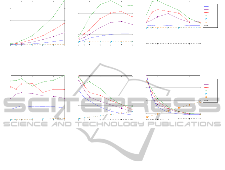
5.2 Control Messages Cost

Figure 5 shows the average number of control mes-

sages sent by nodes. For

of nodes aware of their po-

sition (Fig. 5(a)), we observe for HGA that, the deeper

is the search, the more there is control messages. Like-

wise, the higher is density, the more messages are sent.

It can be explained by the fact that more nodes receive

the RREQs when the density is higher, each node re-

ceiving a RREQ potentially re-emits it, explaining the

exponential increase of the number of messages emit-

ted with the average density. It also explains why the

increase is stronger when the route search if deeper.

Figures show that the number of control messages sent

by Greedy is very low because only nodes aware of

their position emit control messages. For Greedy and

VCap, the number of control messages sent is constant

as it does not depend on density. For a low density, the

control messages number is close for all algorithms.

The gap increases with the density. For low densities,

it is interesting to prefer HGA-

which offers high de-

livery ratio, compared to other solutions, while adding

a reasonable amount of control messages. When the

average density increases, VCap is more suitable as

it offers a delivery ratio close to, if not better than

some variants of HGA while generating less control

messages.

When the number of nodes aware of their posi-

tion increases to

, the number of control messages

strongly decreases for HGA, especially with deep

search. This behavior is explained because the proba-

bility of ﬁnding a route during a RREQ increases when

the number of nodes aware of their position increases.

This probability also increases when the density of

nodes increases (there is more nodes in the neighbor-

hood to satisfy the request). This explains the inversion

of curves for HGA for

and

10%

of nodes aware of

their position (Fig. 5(b) and 5(c)). However, there is

no need to use deep variants for

10%

of nodes aware

of their position as the delivery ratio rapidly reaches

100% in that case.

5.3 Memory Cost

Figure 6 shows memory usage for the different algo-

rithms. We can see that memory needs are much higher

for HGA than VCap when

of nodes are aware of

their position (Fig. 6(a)). With

(Fig 6(b)), the gaps

for memory usage are lower and even really close to

VCap when average density increase. On Figure 6(c),

with

10%

of nodes with position knowledge, memory

needs are much lower for HGA and even lower than

VCap when density is over 40.

The memory size for Greedy is only the number of

neighbors aware of their position for each node. The

high amount of memory needed by HGA is explained

because in simulations, every route is kept until the

end of the simulation. It would be possible to lower

the memory needs by “forgetting” old routes with the

counterpart of having to send more control messages.

We can highlight that experimental conditions are de-

manding concerning memory needs. Indeed, sources

and destinations of data packet are chosen randomly

at a high frequency. In real applications, the number

of destinations of data packets are often limited if not

unique in case of data collection. In case of actuators,

one base station sends messages to different sources.

In that case the source is unique, thus the number of

routes to memorize for each node is reduced.

SENSORNETS2014-InternationalConferenceonSensorNetworks

170

10 20 30 40

50 60

·10

average density

control messages number per node

(a) 1% position aware nodes.

10 20 30 40

50 60

2,000

4,000

6,000

8,000

average density

control messages number per node

(b) 5% position aware nodes.

10 20 30 40

50 60

500

1,000

1,500

average density

control messages number per node

HGA 1

HGA 2

HGA 3

HGA 5

Vcap 3

Vcap 5

Greedy

Figure 5: Message control number.

10 20 30 40

50 60

500

1,000

1,500

average density

memory size

(a) 1% position.

10 20 30 40

50 60

100

200

300

average density

memory size

(b) 5% position.

10 20 30 40

50 60

100

120

average density

memory size

HGA 1

HGA 2

HGA 3

HGA 5

Vcap 3

Vcap 5

Greedy

Figure 6: Average size in memory.

6 CONCLUSIONS

In this article we propose a novel solution for geo-

graphic routing, that allow to use nodes position when

available but also able to deal with unavailable po-

sitions. To the best of our knowledge, there is no

solution in the literature which relies on the same as-

sumptions. Indeed, we can ﬁnd geographic routing

solutions for networks with all nodes aware of their

positions as well as solutions using virtual coordinates

where no node is aware of its position. We propose an

hybrid solution, taking advantages of real node posi-

tion when available but able to operate if not always

available. The geographic and the reactive methods

illustrated in this paper could be replaced by some

other methods from literature or new ones. Both part

should be chosen regarding application needs. The

underlying topology of the application will favor some

geographic routing techniques while the trafﬁc pattern

will favor the classical routing part. For low data rates,

the classical routing part could be proactive or even

hybrid as proposed in ZRP (Haas et al., 2002).

Our solution,

HGA

offers much better perfor-

mances than Greedy geographic routing if part of the

nodes are not aware of their position. We also compare

HGA

with a routing solution based on virtual coordi-

nates, VCap, and show that for different scenarios, our

solution offer better performances with a limited or no

overhead.

For future works, we consider to validate our works

with realistic physical and MAC layers. The use of

real platform such as FIT or SmartSantander (Sanchez

et al., 2011) would allow us to validate these aspects

while testing realistic environments.

Studying node mobility is another interesting as-

pect, we could characterize the needed timeout before

routes expires with regards to nodes speed. Compari-

son with routing algorithm using virtual coordinates

would also bring some arguments for

HGA

since these

algorithms need to frequently rebuild coordinates sys-

tem, and then, increase number of control messages

exchanged in the network.

Finally it could be interesting to compare our solu-

tion with a variant in which each node keeps a

-hop

neighborhood table instead of using

-hop RREQ. The

study of control messages number would allow us to

ﬁnd threshold to know which variant is better in some

cases.

REFERENCES

Al-Hader, M., Rodzi, A., Sharif, A., and Ahmad, N. (2009).

Smart City Components Architecture. In Proceedings

GeographicRoutingwithPartialPositionInformation

171

of the International Conference on Computational In-

telligence, Modelling and Simulation, CSSim, pages

93–97, Brno, Czech Republic. IEEE.

Capkun, S., Hamdi, M., and Hubaux, J.-P. (2002). GPS-

free Positioning in Mobile Ad Hoc Networks. Cluster

Computing, 5(2):157–167.

Benbadis, F., Puig, J.-J., de Amorim, M. D., Chaudet, C.,

Friedman, T., and Simplot-Ryl, D. (2006). Jumps: En-

hancing hop-count positioning in sensor networks us-

ing multiple coordinates. International Journal on Ad

Hoc and Sensor Wireless Networks, abs/cs/0604105.

Benkic, K., Malajner, M., Planinsic, P., and Cucej, Z. (2008).

Using RSSI value for distance estimation in wireless

sensor networks based on ZigBee. In Proceedings

of the 15th International Conference on Systems, Sig-

nals and Image Processing, IWSSIP, pages 303–306,

Bratislava, Slovakia.

Caruso, A., Chessa, S., De, S., and Urpi, A. (2005). GPS

free coordinate assignment and routing in wireless sen-

sor networks. In Proceedings of the 24th Annual Joint

Conference of the IEEE Computer and Communica-

tions Societies, INFOCOM, pages 150–160, Miami,

FL, USA. IEEE.

avez, E., Mitton, N., and Tejeda, H. (2007). Routing in

Wireless Networks with Position Trees. In Kranakis,

E. and Opatrny, J., editors, Ad-Hoc, Mobile, and Wire-

less Networks, ADHOC-NOW, pages 32–45, Cancun,

Mexico. Springer Berlin Heidelberg.

Elhafsi, E. H., Mitton, N., and Simplot-Ryl, D. (2007). Cost

over Progress Based Energy Efﬁcient Routing over

Virtual Coordinates in Wireless Sensor Networks. In

Proceedings of International Symposium on a World

of Wireless, Mobile and Multimedia Networks, WoW-

MoM, pages 1–6, Helsinki, Finland. IEEE.

Ermel, E., Fladenmuller, A., Pujolle, G., and Cotton, A.

(2005). On Selecting Nodes to Improve Estimated

Positions. In Proceedings of the 7th international Mo-

bile and Wireless Communication Networks, MWCN,

pages 449–460, Marrakech, Morocco. Springer US.

Fang, Q., Gao, J., Guibas, L., de Silva, V., and Zhang, L.

(2005). GLIDER: gradient landmark-based distributed

routing for sensor networks. In Proceedings of the

24th Annual Joint Conference of the IEEE Computer

and Communications Societies, INFOCOM, pages 339–

350, Miami, FL, USA. IEEE.

Fraboulet, A., Chelius, G., and Fleury, E. (2007). Worldsens:

Development and Prototyping Tools for Application

Speciﬁc Wireless Sensors Networks. In Proceedings

of the 6th International Symposium on Information

Processing in Sensor Networks, IPSN, pages 176–185,

Cambridge, MA, USA. ACM.

Haas, Z. J., Pearlman, M. R., and Samar, P. (2002). The

Zone Routing Protocol (ZRP) for Ad Hoc Networks.

IETF Internet Draft.

Liu, K. and Abu-Ghazaleh, N. (2008). Stateless and guaran-

teed geometric routing on virtual coordinate systems.

In Proceedings of the 5th International Conference

on Mobile Ad Hoc and Sensor Systems, MASS, pages

340–346, Atlanta, GA, USA. IEEE.

Mitton, N., Razaﬁndralambo, T., Simplot-Ryl, D., and Stoj-

menovic, I. (2012). Towards a hybrid energy efﬁcient

multi-tree-based optimized routing protocol for wire-

less networks. Sensors, 12(12):17295–17319.

Niculescu, D. and Nath, B. (2001). Ad hoc positioning sys-

tem (APS). In Proceedings of the Global Telecommuni-

cations Conference, GLOBECOM, pages 2926–2931,

San Antonio, TX, USA. IEEE.

Perkins, C. and Royer, E. (1999). Ad-hoc on-demand

distance vector routing. In Proceedings of the 2nd

Workshop on Mobile Computing Systems and Appli-

cations, WMCSA, pages 90–100, New Orleans, LA,

USA. IEEE.

Sanchez, L., Galache, J., Gutierrez, V., Hernandez, J., Bernat,

J., Gluhak, A., and Garcia, T. (2011). Smartsantander:

The meeting point between future internet research and

experimentation and the smart cities. In Future Net-

work Mobile Summit, FutureNetw, pages 1–8, Warsaw,

Poland.

Seada, K., Helmy, A., and Govindan, R. (2004). On the

effect of localization errors on geographic face routing

in sensor networks. In Proceedings of the 3rd interna-

tional symposium on Information processing in sensor

networks, IPSN, pages 71–80, New York, NY, USA.

ACM.

Stojmenovic, I. (2006). Localized network layer protocols

in wireless sensor networks based on optimizing cost

over progress ratio. IEEE Network, 20(1):21–27.

SENSORNETS2014-InternationalConferenceonSensorNetworks

172