Fast Incremental Objects Identification and Localization using
Cross-correlation on a 6 DoF Voting Scheme
Mauro Antonello, Alberto Pretto and Emanuele Menegatti
University of Padova, Dep. of Information Engineering (DEI)
via Gradenigo 6/B, 35131 Padova, Padova, Italy
Keywords:
Gaussian Mixtures, Online Learning, Pose Estimation, Object Recognition.
Abstract:
In this work, we propose a sparse features-based object recognition and localization system, well suited for
online learning of new objects. Our method takes advantages of both depth and ego-motion information,
along with salient feature descriptors information, in order to learn and recognize objects with a scalable ap-
proach. We extend the conventional probabilistic voting scheme for object the recognition task, proposing a
correlation-based approach in which each object-related point feature contributes in a 6-dimensional voting
space (i.e., the 6 degrees-of-freedom, DoF, object position) with a continuous probability density distribution
(PDF) represented by a Mixture of Gaussian (MoG). A global PDF is then obtained adding the contribution of
each feature. The object instance and pose are hence inferred exploiting an efficient mode-finding method for
mixtures of Gaussian distributions. The special properties of the convolution operator for the MoG distribu-
tions, combined with the sparsity of the exploited data, provide our method with good computational efficiency
and limited memory requirements, enabling real-time performances also in robots with limited resources.
1 INTRODUCTION
The object recognition task has received consider-
able attention in the computer vision community dur-
ing the last decade, by paying attention especially to
general object categorization starting from a limited
amount of instances and providing many benchmarks
on public datasets. On the other hand, object recog-
nition in robotics usually needs to deal with specific
instances of an object. Moreover, robots often need
to manipulate the found object, so an accurate local-
ization of the object of interest is desirable. The So-
lutions in Perception Challenge (Marvel et al., 2012),
held at ICRA in 2011, highlighted the specific prob-
lems of the object recognition task inside the robotic
domain, by focusing on the objects instances identifi-
cation and localization problems.
Robots are usually equipped with many sensors in ad-
dition to the camera, that could be actively exploited
in the object recognition task. RGB-D sensors as the
Kinect system or a RGB-D camera enable better 3D
object localization ((Tang and Miller, 2012; Lai et al.,
2011b; Xie et al., 2013; Wohlkinger et al., 2012)),
inertial measurements units, joined with vision, can
provide accurate ego-motion estimation (e.g., (Tsot-
sos et al., 2012)) enabling the robot with active vi-
sion capabilities that help to increase the confidence
in the object classification. Actually, state of the
art systems (among others, (Tang and Miller, 2012;
Vaskevicius and Pathak, 2012)) usually face these
problems collecting dense point clouds of the objects
(depths and point color), taken from multiple views
during the training step. A 3D full model is hence
built offline from the clouds set. During the online
recognition step, the built models are matched against
the current point cloud using 3D descriptors such as
the VHF and the FPFH features ((Rusu and Brad-
ski, 2010; Rusu, 2009)). Local image feature can be
used to help the recognition and enforce constraints
in the localization ((Tang and Miller, 2012; Vaskevi-
cius and Pathak, 2012)). Despite that such a systems
perform so well in unstructured benchmarking scene,
they suffer some disadvantages. Usually, they require
to learn full 3D models of the objects during the train-
ing stage, and making it difficult to learn new, possi-
bly incomplete, objects online. Moreover, for identi-
fication purposes, occlusions are usually handled bet-
ter by using local image descriptors instead of dense
but incomplete point clouds. Finally, deal with dense
point clouds usually requires much higher computa-
tional effort and memory requirements compared with
sparse points approaches.
499
Antonello M., Pretto A. and Menegatti E..
Fast Incremental Objects Identification and Localization using Cross-correlation on a 6 DoF Voting Scheme.
DOI: 10.5220/0004873604990504
In Proceedings of the 9th International Conference on Computer Graphics Theory and Applications (WARV-2014), pages 499-504
ISBN: 978-989-758-002-4
Copyright
c
 2014 SCITEPRESS (Science and Technology Publications, Lda.)

2 THE PROPOSED METHOD
In order to recognize known objects during normal
operation, our system should be trained with a set
of the objets of interest, i.e. we need to populate a
database with the models of these objects. The pro-
posed method describes the known objects by means
of a set of statistical distribution of the object visual
features, that embeds also structure information as
the keypoint locations and the view-point from which
they are extracted.
Given an object of interest, we collect a set of im-
ages, depth maps and view points tuples {I
i
,D
i
,ω
i
},
where ω
i
∈ R
3
is the orientation vector of the view-
point from which the image I
i
is taken and D
i
is
the depth image. We can express a rigid body trans-
formation g = [T|Ω] ∈ SE(3) in terms of a transla-
tion vector T = [t
x
t
y
t
z
]
T
and a orientation vector
Ω = [r
x
r
y
r
z
]
T
, both in R
3
. We make explicit this
fact using the notation g(T,Ω) = g. R(Ω)
.
= exp(
b
Ω)
is the rotation matrix corresponding to the rotation
vector Ω, where
b
Ω is the skew-symmetric matrix cor-
responding to Ω, and Log
SO(3)
(R(Ω))
.
= Ω is the ro-
tation vector Ω corresponding to the rotation matrix
R(Ω). A feature detector (e.g., SIFT features) is then
run over each image I
i
to extract a set of keypoints
and the relative descriptors {k
i
j
,d
i
j
}, with k
i
j
∈ R
6
the 6 DoF coordinates of the extracted keypoint and
d
i
j
the descriptor tuple. The keypoint 3D position is
extracted from the depth map D
i
and its 3D orien-
tation is obtained through cross product of the SIFT
orientation with the normal to the keypoint surface
patch. Each collected keypoint k
i
j
in the image in I
i
votes for a 6 DoF object position v
i
j
expressed by:
v
j
i
= (−k
i
j
)(c
i
,ω
i
)
where c
i
∈ R
3
are the 3D coordinates of the object
center (computed as the centroid of the point cloud).
For the sake of efficiency, and to reduce the number
of distributions that compose an object model, we
clusterize the visual descriptors d
i
j
into simpler visual
words. The Bag-of-Words {w
k
}
k=1..N
we employ is
created using the k-means clustering method from a
large and random set of feature descriptors, extracted
from a set of natural images. In this way, keypoint
with descriptors close to others are expressed by a
single visual word w
k
grouped together in order
to populate a single 6 dimensional voting space V
k
represented by a Mixture of Gaussian distribution:
each object position hypothesis v
j
i
contributes to gen-
erate this multi-modal PDF. The MoG is efficiently
computed online using an integration-simplification
based method (see Sec. 2.1). When a new keypoint
along with its voting position v
j
i
is extracted, the
visual words w
k
nearest to d
i
j
is searched. In case of
success, v
j
i
will contribute to modify the voting space
V
k
as described in Sec. 2.1. To improve recognition
performances, a vote v
j
i
is generated only if the
assignment of d
i
j
to w
k
is not ambiguous. Let be
w
k
1
,w
k
2
the two nearest words to d
i
j
and let be
d
h
= |d
i
j
−w
k
h
|
2
their distances, v
j
i
is accepted only
if
d
2
d
1
> 0.8. At the end of the training step, each
object model contains N voting spaces V
k
(MoG),
one for each visual word w
k
.
During the online recognition step, the process de-
scribed above is used to dynamically create a model
of the scene M
S
, using as input frames gathered by
RGB-D camera and poses obtained through a struc-
ture from motion algorithm. After each update, a set
of candidate object models M
O
i
is selected from all
learned object models. The candidates set includes all
models that contain a non empty MoG for at least one
of the visual words detected in the last video frames.
Each candidate model M
O
h
is then matched against
M
S
to verify if the object is actually present in the
scene, and where. To figure out if M
O
h
is embedded
in M
S
, and to evaluate the best embedding points p
h
,
for each visual word we select from the two models
M
O
h
and M
S
the corresponding MoGs. Then, we
compute their Cross-Correlation MoG as described in
Sec. 2.2. The result of this operation is a set of MoGs
that are merged together. We apply a mode finding al-
gorithm to this final MoG and the modes actually rep-
resents embedding points p
h
. The points p
h
are con-
sidered as insights of the possible locations of M
O
in
M
S
, their embedding quality is the actual probability
of these guesses.
2.1 MoG Online Training
The most common method for fitting a set of data
points (in our case, the object position v
j
i
) with a
MoG is based on Expectation Maximization (Demp-
ster et al., 1977). Unfortunately, this is an offline
method and does not suit for a scenario in which
new data comes continuously (i.e., new keypoints)
and can’t be stored indefinitely. Many solutions have
been proposed to address this issue (Hall et al., 2005)
(Song and Wang, 2005) (Ognjen and Cipolla, 2005),
but most of them are based on the split and merge
criterion and they are too slow or constrained for
our application. In order to fit the objects position
with a MoG, we employ a continuous integration-
simplification loop that relies on a fidelity criterion
to guarantee the required accuracy (Declercq and Pi-
GRAPP2014-InternationalConferenceonComputerGraphicsTheoryandApplications
500

ater, 2008). Let be f
t
(x) the PDF of a MoG already
learned from data up to time t:
w
t
i
∈ R, x, µ
t
i
∈ R
n
, Σ
t
i
∈ R
nxn
,
X
t
i
= N (µ
t
i
,Σ
t
i
)f
t
(x) =
N
X
i=1
w
t
i
p
X
t
i
(x),
N
X
i=1
w
t
i
= 1
Where w
t
i
,µ
t
i
and Σ
t
i
are respectively the weight,
mean and the covariance of the Gaussian components
of MoG. If at this time new data needs to be inte-
grated, a new component X
t
i+1
is learned from it and
merged into the old MoG. Similarly to (Hall et al.,
2005), our update process is done in two steps:
1. Concatenate: trivially add X
t
i+1
to produce a
new MoG with N + 1 components.
2. Simplify: if possible, merge some components to
reduce the MoG complexity. This is done through
the fidelity criterion proposed by (Declercq and
Piater, 2008).
2.2 Cross-Correlation (CC) on MoGs
Figure 1: The Cross-Correlation MoG presents a clear peak
to the displacement value between MoG
B
and MoG
A
. The
peak value is proportional to the similarity between the
source MoGs.
The key idea underlying our recognition and lo-
calization process is the tight connection between the
Cross-Correlation (CC) and the Convolution opera-
tors. Actually, the CC of two real continuous func-
tions, f
1
(t) and f
2
(t), is equivalent to the convolution
of f
1
(−t) and f
2
(t). In our work, the CC operates on
two MoGs achieving two key results at the same time:
peaks in the CC function provides both the maximum
registration locations and quality (Fig. 1). Calculating
the CC of two MoGs is a fast operation thanks to the
closure of Gaussian functions respect to the convolu-
tion operation. Given the PDFs of two Multivariate
Normal distributions:
x, µ
i
∈ R
n
, Σ
i
∈ R
nxn
X
1
= N (µ
1
,Σ
1
), X
2
= N (µ
2
,Σ
2
)
f
i
(x) =
1
p
(2π)
k
|Σ
i
|
e
−
1
2
(x−µ
i
)
0
Σ
−1
i
(x−µ
i
)
their convolution:
(f
1
∗ f
2
)(x) =
Z
R
n
f
1
(τ ) f
2
(x − τ )dτ
=
1
p
(2π)
k
|Σ
c
|
e
−
1
2
(x−µ
c
)
0
Σ
−1
c
(x−µ
c
)
(1)
is another Multivariate Normal distributed PDF, with
µ
c
= µ
1
+ µ
2
and Σ
c
= Σ
1
+ Σ
2
. Furthermore, the
distributivity property of the convolution leads to a
closed form for MoGs cross-Correlation. Let be f
A
and f
B
the PDFs of two MoG learned from objects A
and B
f
A
(x) =
N
X
i=1
w
A
i
f
A
i
(x) f
B
(x) =
M
X
j=1
w
B
j
f
B
j
(x)
with
P
N
i=1
w
A
i
= 1 and
P
M
j=1
w
B
j
. Their convolution
is
f
CC
(x) := (f
A
∗ f
B
)(x) =
N
X
i=1
M
X
j=1
w
A
i
w
B
j
f
A
i
(x) ∗ f
B
j
(x).
(2)
With
P
N
i=1
P
M
j=1
w
A
i
w
B
j
= 1. Accordingly, the
CC of two MoG is still a MoG with N M components.
For every possible roto-translation x, f
CC
(x) is pro-
portional to the registration quality of B, rotated and
translated by x, into A.
To find peaks in f
CC
(x) we applied an efficient mode
finding algorithm for MoGs proposed in (Carreira-
Perpinan, 2000).
2.3 Identification and Localization
During the identification process, a scene model is
built online integrating in its MoG all the keypoints
detected while the robot is moving. Every new key-
point is integrated in the MoG associated to the visual
word nearest to the keypoint descriptor. In our exper-
iments, the roto-translation component of these key-
points is obtained by a PCL implementation of the
Microsoft KinectFusion structure from motion tool.
At every fixed amount of time, a first candidates set
{O
i
} of detected objects is created selecting from the
learnt object those models that contains descriptors
FastIncrementalObjectsIdentificationandLocalizationusingCross-correlationona6DoFVotingScheme
501

that are visible in the last images processed. Each
object O
i
is then checked computing the CC be-
tween its MoGs and the correspondent MoGs of the
whole scene model, without requiring a prior seg-
mentation. The resulting MoGs are then fused in a
single MoG, that represents a global distribution of
the object points votes. Peaks {x
j
}
1..k
found in this
resulting MoG are are hypotheses of O
i
locations in
the scene; a peak {x
j
} is considered a valid detection
guess if f
CC
(x
j
) > α
i
. Threshold values α
i
are cal-
culated for every O
i
, and they are proportional to the
complexity of the correspondent MoG. This threshold
has been introduced to normalize peaks obtained reg-
istering MoGs relative to objects with different tex-
ture complexities.
2.4 Handling Data on the 6 DoF
Manifold
Both MoG learning and mode finding normally relies
on the Euclidean distance between data points, and
it needs to be slightly adapted to work with 6 DoF
points. The rotation subspace of the 6 DoF space is a
general manifold, so algorithms proposed so far are
accurate as long as the points involved are near in
the geodesic. To avoid degenerations and loss of pre-
cision when points are far away from others, in the
MoG learning process we have introduced a cap for
the eigenvalues allowed in the components of the co-
variance matrix.
3 EXPERIMENTS
We have implemented all the algorithm described
above inside the ROS framework, using standard vi-
sion and math libraries such as OpenCV, PCL and
Eigen. The choice of such a framework comes from
the objective to obtain the most possible sharable
code, even if some built implementations performs
not so well compared to other external implementa-
tions. The experiments has been performed using a
low cost PC equipped with an Intel Core 2 Duo CPU
(2 GHz) and 2 GB of RAM.
3.1 Dataset
As described above, to integrate new features in a
model, the proposed method makes use of mutual
pose information between the viewer and the object.
In order to fulfill these requirements, we have cho-
sen to evaluate our system on the public RGB-D Ob-
ject Dataset presented in (Lai et al., 2011a), a multi-
view and multi-instance set of images built through
the Kinect sensor from common household objects.
Object views comes from video sequences, in which
the objects are placed on a turntable and filmed for
a whole rotation at three different heights. In some
cases the objects in the images were too small, so the
used feature extraction algorithms didn’t give enough
valid keypoints: we have discarded these instances
from the dataset.
3.2 Instance Recognition
As preliminary step, the Bag of Visual Words has
been built clustering 100k SIFT descriptors extracted
from the whole background scenes dataset. We used
the classic k-means method to obtain a visual vocab-
ulary with 200 words. During the model creation pro-
cess, keypoints contribute with a vote only if their de-
scriptor’s nearest visual word were at least 20% closer
then the second.
Train object models are created with all frames in the
RGB-D dataset but for evaluation models only a small
subset is used, as suggested by dataset providers we
kept only one frame every five. To simulate an online
train process, frames are added to models at the rate
of 10 frames per second. Every evaluation model is
then compared to all trained models, estimating the
similarity index and the relative pose at the same time
(Fig. 2. The instance recognition rate of our method
is on average 77.3%; most of unrecognized instances
are due to a smaller area of the object in its images or
presence of light reflections.
3.3 Pose Recognition
The evaluation of the pose error is achieved by com-
parison of two models of the same instance type,
which pose were known a priori. The difference
from the resulting pose and the ground truth is then
recorded for both translation an rotation values. Eval-
uation models has been rotated an translated with a
random position before the recognition phase. In gen-
eral results showed that our method can recognize the
pose with high precision (Fig. 3), however objects
presenting high texture symmetries often led to higher
localization errors.
4 CONCLUSIONS AND FUTURE
WORKS
We have shown that MoG-based object modeling and
the Cross-Correlation operator between MoGs can
be reliable and fast tools to represent, recognize and
GRAPP2014-InternationalConferenceonComputerGraphicsTheoryandApplications
502

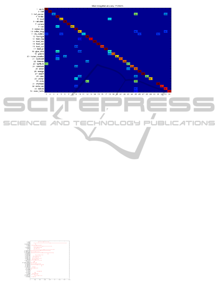
Figure 2: Confusion matrix: instance recognition rates of each object class.
locate objects. The convolution operator, and con-
sequently the Cross-Correlation, can advantage the
same closure properties also with different structures
based on Gaussians or Fourier Transform. We will
further analyze these structures to improve the com-
parison performances and speed. Some limitations of
our approach come from the fact that we have used 2D
SIFT keypoints, where in many cases objects were too
small to obtain a good number of keypoints or, even
worse, light reflections and low textures generated
keypoints with low discriminative power. Such key-
points lead to distributions that poorly describe object
appearance; an easy and effective improvement of our
system will be the integration of different types of
keypoint detectors (possibly 3D). Another challenge
will be a more precise management of the algorithms
in the 6 DoF manifold, this requires an accurate op-
timization of the code to maintain real time perfor-
mances.
Figure 3: Norm means and standard deviations of the dif-
ferences between the 6DoF ground truth pose and the esti-
mated one. Only good matches contribute to the statistic.
REFERENCES
Carreira-Perpinan, M. (2000). Mode-finding for mixtures
of Gaussian distributions. Pattern Anal. Mach. Learn.,
pages 1–23.
Declercq, A. and Piater, J. H. (2008). Online learning of
gaussian mixture models: a two-level approach.
Dempster, A., Laird, N., and Rubin, D. (1977). Maxi-
mum likelihood from incomplete data via the EM al-
gorithm. J. R. Stat. Soc., 39(1):1–38.
Hall, P., Hicks, Y., and Robinson, T. (2005). A method to
add Gaussian mixture models.
Lai, K., Bo, L., Ren, X., and Fox, D. (2011a). A large-scale
hierarchical multi-view RGB-D object dataset. ICRA,
pages 1817–1824.
Lai, K., Bo, L., Ren, X., and Fox, D. (2011b). Sparse dis-
tance learning for object recognition combining RGB
and depth information. ICRA, (1):4007–4013.
Marvel, J. a., Hong, T.-H., and Messina, E. (2012). 2011
Solutions in Perception Challenge Performance Met-
rics and Results. Proc. Work. Perform. Metrics Intell.
Syst. - Permis ’12, page 59.
Ognjen, A. and Cipolla, R. (2005). Incremental Learning of
Temporally-Coherent Gaussian Mixture Models.
Rusu, R. and Bradski, G. (2010). Fast 3d recognition and
pose using the viewpoint feature histogram. Intell.
Robot. . . . , pages 2155–2162.
Rusu, R. B. (2009). Fast Point Feature Histograms (FPFH)
for 3D registration. Robot. Autom. 2009. . . . , pages
3212–3217.
Song, M. and Wang, H. (2005). Highly efficient incremental
estimation of Gaussian mixture models for online data
stream clustering. pages 174–183.
Tang, J. and Miller, S. (2012). A textured object recogni-
tion pipeline for color and depth image data. Robot.
Autom.
Tsotsos, K., Pretto, A., and Soatto, S. (2012). Visual-
Inertial Ego-Motion Estimation for Humanoid Plat-
FastIncrementalObjectsIdentificationandLocalizationusingCross-correlationona6DoFVotingScheme
503

forms. In IEEE-RAS Int. Conf. Humanoid Robot.,
pages 704–711.
Vaskevicius, N. and Pathak, K. (2012). The jacobs robotics
approach to object recognition and localization in the
context of the ICRA’11 Solutions in Perception Chal-
lenge. Robot. Autom. . . . , pages 3475–3481.
Wohlkinger, W., Aldoma, A., Rusu, R. B., and Vincze, M.
(2012). 3DNet: Large-scale object class recognition
from CAD models. ICRA, pages 5384–5391.
Xie, Z., Singh, A., Uang, J., Narayan, K., and Abbeel, P.
(2013). Multimodal Blending for High-Accuracy In-
stance Recognition. IROS.
GRAPP2014-InternationalConferenceonComputerGraphicsTheoryandApplications
504