
Evaluating Artificial Neural Networks and Traditional Approaches for
Risk Analysis in Software Project Management
A Case Study with PERIL Dataset
Carlos H. M. S. Timoteo, Meuser J. S. Valenca and Sergio M. M. Fernandes
Computer Engineering Department, University of Pernambuco, Rua Benfica, Recife, Brazil
Keywords:
Software Project, Risk Management, Risk Analysis, Support Vector Machine, MultiLayer Perceptron, Monte
Carlo Simulation, Linear Regression Model.
Abstract:
Many software project management end in failure. Risk analysis is an essential process to support project
success. There is a growing need for systematic methods to supplement expert judgment in order to increase
the accuracy in the prediction of risk likelihood and impact. In this paper, we evaluated support vector machine
(SVM), multilayer perceptron (MLP), a linear regression model and monte carlo simulation to perform risk
analysis based on PERIL data. We have conducted a statistical experiment to determine which is a more
accurate method in risk impact estimation. Our experimental results showed that artificial neural network
methods proposed in this study outperformed both linear regression and monte carlo simulation.
1 INTRODUCTION
How risky are software projects? Several studies
about effectiveness of software cost, scope, schedule
estimation techniques; surveys from software profes-
sionals in industry; and analysis of project portfolios
have been done to answer this question (Budzier and
Flyvbjerg, 2013). However, there is not a consensus.
Some authors (Schmidt et al., 2001) have noticed
that many software development projects end in fail-
ure. They showed that around twenty five percent
of all software projects are canceled outright and as
many as eighty percent of all software projects run
over their budget, exceeding it by fifty percent in av-
erage. Industry surveys suggest that only a quarter
of software projects succeed outright, and billions of
dollars are lost annually through project failures or
projects that do not deliver promised benefits (Ban-
nerman, 2008). Moreover, that study showed evi-
dences that it’s a global issue, impacting private and
public sector organizations.
Risk can be defined as the possibility of loss or in-
jury (Boehm, 1991). This definition can be expressed
by risk exposure formula. This study takes into a def-
inition whereupon project risk is a certain event or
condition that, if it occurs, has a positive or nega-
tive effect on one or more project objectives (Institute,
2008). A complement that definition risk is a mea-
sure of the probability and severity of adverse effects
(Haimes, 2011).
A limitation can be found in Boehm’s risk defini-
tion - it is very difficult, in practice, to estimate the
probability of many risk factors, especially in soft-
ware projects (Bannerman, 2008). Probability and
impact can only be meaningfully determined for ac-
tivities that are repeated many times, under controlled
circumstances, so the one-off nature of many software
project activities mitigates accurate estimates.
So, there is an increasing need for more systematic
methods and tools to supplement individual knowl-
edge, judgment, and experience. Human traits are
often sufficient to address less complex and isolated
risks. For example, a portion of the most serious is-
sues encountered in system acquisition are due to ig-
nored risks under low likelihood, until they create se-
rious consequences (Higuera and Haimes, 1996).
Monte Carlo Simulation (MCS) is cited as a good
method for project risk analysis (Institute, 2008).
However, there are some limitations that becomes
it unfeasible (Support, 2005). Simulations can lead
to misleading result if inappropriate inputs, derived
from subjective parametrization, are entered into the
model. Commonly, the user should be prepared to
make the necessary adjustments if the results that are
generated seem out of line. Moreover, Monte Carlo
can not model risks correlations. It means that num-
bers coming out in each draw are random, in conse-
quence, an outcome can vary from its lowest value,
472
Timoteo C., Valença M. and Fernandes S..
Evaluating Artificial Neural Networks and Traditional Approaches for Risk Analysis in Software Project Management - A Case Study with PERIL Dataset.
DOI: 10.5220/0004885704720479
In Proceedings of the 16th International Conference on Enterprise Information Systems (ICEIS-2014), pages 472-479
ISBN: 978-989-758-027-7
Copyright
c
2014 SCITEPRESS (Science and Technology Publications, Lda.)

in one period, to the highest in the next. Therefore,
alternative approaches must be investigated to predict
risks.
The main purpose of this paper is to analyze which
is a more efficient approach to software project risk
analysis: MCS technique or Artificial Neural Net-
works (ANN’s) alternatives, through Multilayer Per-
ceptron (MLP) and Support Vector Machine (SVM),
to improve accuracy and decrease error prone. A Lin-
ear Regression Model (LRM) is also considered as
baseline during the method.
The methodology adopted in this study is a sta-
tistical experiment to evaluate the prediction error of
risk impact from PERIL dataset (Kendrick, 2003), a
framework to identify risks in software project man-
agement. The four selected techniques must estimate
the outcome to risk impacts. Mean Absolute Error
(MAE) will be calculated thirty times for each ap-
proach, and then a hypothesis test may be necessary
to achieve the study goal.
Section 2 presents basic concepts to perform the
experiment. Section 3 presents the methodology for
this study, including dataset characterization. Section
4 presents the result analysis and establishes the best
analyzed technique. In the end, Section 5 concludes
this work and presents limitations and future works.
2 STATE OF ART
After a short bibliographic revision, we have identi-
fied numerous alternative approaches to risk analy-
sis, which includes Bayesian Belief Networks, Arti-
ficial Neural Networks (ANN), Decision Tree (DT),
Fuzzy Set Theory (FST), Neuro-Fuzzy System (NFS)
(Huang et al., 2004) (Hu et al., 2007) (Attarzadeh and
Ow, 2010) (Dzega and Pietruszkiewicz, 2010) (Yu,
2011) (Saxena and Singh, 2012) (Dan, 2013).
Genetic algorithm was utilized to improve ANN
estimator (Hu et al., 2007). Experimental results
showed that it achieved higher accuracy when com-
pared to a SVM model. Moreover, a proposed
ANN model that incorporates with Constructive Cost
Model (COCOMO) was improved through particle
swarm optimization, to estimate the software devel-
opment effort accurately. Another authors improved
cost estimation for COCOMO’81, towards a gen-
eral framework for software estimation based on NFS
(Huang et al., 2004).
A model based on fuzzy theory have overcome the
difficulty of qualitative and quantitative assessment of
traditional methods (Yu, 2011). Neuro-fuzzy tech-
niques also was explored to design a suitable model
to improve software effort estimation for NASA soft-
ware projects, on purpose a NFS had the lowest pre-
diction error compared to existing models (Saxena
and Singh, 2012).
Results from risk analysis experiments performed
through data mining classifiers - C4.5, RandomTree,
classification and regression tree algorithms - have
been presented (Dzega and Pietruszkiewicz, 2010).
The authors described how boosting and bagging
metaclassifiers were applied to improve the outcomes,
but also have analyzed influence of their parameters
on generalization and in prediction accuracy. Al-
though, the authors rejected MLP and SVM prema-
turely.
2.1 Project Risk Management
According to PMI (Institute, 2008), project risk man-
agement includes planning, identification, analysis,
response planning, monitoring and controlling risks.
Its purpose is to increase likelihood and impact of
positive events and reduce probability and severity
of negative events. From management point of view,
making informed decisions by consciously assessing
what can go wrong, as well as its likelihood and sever-
ity of the impact, is at the heart of risk management.
Project risk management processes are:
• Planning risk management: The process of defin-
ing how conduct risk management activities;
• Identifying risks: The process of determining
risks that can affect project and documenting its
characteristics;
• Performing qualitative risk analysis: The process
of prioritizing risks to analyze through assessment
and combination of its occurrence probability and
impact;
• Performing quantitative risk analysis: The pro-
cess of analyzing numerically the effect of pre-
vious identified risks, in terms of general project
objectives;
• Planning risk responses: The process of develop-
ing options and actions to increase opportunities
and decrease threats to project objetives;
• Monitoring and controlling risks: The process of
implementing risk responses planning, tracking
identified risks, monitoring residual risks, identi-
fying new risks and assessing the efficacy of risk
treatment process during the whole project.
2.1.1 Risk Analysis
Analysis is the conversion of risk data into risk
decision-making information. Analysis provides the
basis for the project manager to work on the most
EvaluatingArtificialNeuralNetworksandTraditionalApproachesforRiskAnalysisinSoftwareProjectManagement-A
CaseStudywithPERILDataset
473

critical risks. Boehm (1991) defines risk analysis ob-
jective as the assessment of the loss probability and
magnitude for each identified risk item, and it as-
sesses compound risks in risk-item interactions. Typ-
ical techniques include performance and cost mod-
els, network analysis, statistical decision analysis and
quality-factor (like reliability, availability, security)
analysis.
Risk analysis depends on a good mechanism to
identify risks. However, most of the methods as-
sume that managers have the required experience to
be aware of all pertinent risk factors, but it can not be
the situation. Moreover, many of these methods can
be time-consuming and thus too costly to use on a reg-
ular basis. Therefore, one popular method for identi-
fying risk factors has been the use of checklists. Un-
fortunately, these checklists are based in small sam-
ples or, even worse, flawed in their risk historical data
collection methods.
PMI (Institute, 2008) cites sensibility analysis,
earned monetary value (EMV), modeling and simu-
lation, specialized opinion as most used techniques.
2.1.2 Monte Carlo Simulation
Monte Carlo simulation is a technique that computes
or iterates the project cost or schedule many times
using input values selected at random from probabil-
ity distributions of possible costs or durations, to cal-
culate a distribution of possible total project cost or
completion dates (Institute, 2008).
A model is developed, and it contains certain in-
put variables. These variables have different possible
values, represented by a probability distribution func-
tion of the values for each variable. The Monte Carlo
method is a detailed simulation approach through in-
tensive computing to determine the likelihood of pos-
sible outcomes of a project goal; for example, the
completion date. The inputs of the procedure are ob-
tained randomly from specific intervals with probabil-
ity distribution functions for the durations of schedule
activities or items from cost baseline. Those differ-
ent input values are used to construct a histogram of
possible results to the project and its relative prob-
ability, but also the cumulative probability to calcu-
late desired contingency reserves for time or cost.
Additional results include the relative importance of
each input in determining the overall project cost and
schedule (Kwak and Ingall, 2007).
2.2 Artificial Neural Networks
An ANN is a massively parallel distributed proces-
sor made up of simple processing units, which has
a natural propensity (Haykin, 1994). It adopts non-
parametric regression estimates made up of a number
of interconnected processing elements between input
and output data.
2.2.1 MultiLayer Perceptron
MLP model is constituted of some neurons organized
in at least three layers. The first of them is the input
layer, in which input variables are directly connected
to a exclusive neuron. The next is the hidden layer
that completely connects the neurons from previous
layer to the neurons in output layer. Lastly, output
layer represents ANN outcome. Each input in a neu-
ron has an associated weight to be adjusted by training
algorithm. Common MLP models contain one bias
neuron. MLP is a direct graph, in which inputs data
are propagated from input layer to hidden layers and
from hidden layers to output layer. The data flow in
forward way is known as ”forward phase”. The data
flow in the opposite way is the ”backward phase”.
One major concern of ANN is the stability-
plasticity dilemma. Although continuous learning is
desired in ANN, further learning will cause the ANN
to lose memory when the weights have reached a
steady state (Haykin, 1994). The Backpropagation al-
gorithm is used as training method because it allow
us to adjust weights of multilayer networks, towards
Generalized Delta Rule (Rumelhart et al., 1985).
2.2.2 Support Vector Machine
Support Vector Machine (SVM) is an elegant tool for
solving pattern recognition and regression problems.
It has attracted a lot of attention from researchers due
to its ability to provide excellent generalization per-
formance. The goal of SVM regression is to estimate
a function that is as ”close” as possible to the target
outcomes for every input data in training set and at
the same time, is as ”flat” as possible for good gen-
eralization. More details about SVM can be found in
(Shevade et al., 1999).
3 METHODOLOGY
In this paper, we analyzed which is a more efficient
approach to risk analysis of software projects: MCS,
MLP, SVM or a LRM. A LRM was considered as
baseline approach. The analysis was made in terms
of prediction accuracy. Accuracy means the degree of
closeness of a predicted outcome to the true value. A
metric of accuracy is the Mean Absolute Error (MAE)
given by
ICEIS2014-16thInternationalConferenceonEnterpriseInformationSystems
474

MAE =
1
n
n
∑
i=1
|e
i
|, (1)
where e
i
= f
i
− y
i
, f
i
is the calculated outcome, y
i
is the expected outcome and n is the number of data
pairs.
The four selected techniques have predicted the
outcome to risk impacts. Mean Absolute Error was
calculated thirty times for each method. Neverthe-
less, a Non-paired Wilcoxon Test (Siegel, 1956) may
be necessary to assert which is a more efficient ap-
proach to fit PERIL. Non-paired Wilcoxon Test is
used because there were no evidence that the samples
came from a normally distributed population, either
there were no relation between outcomes from differ-
ent samples.
One important requirement considered in this
study is that the same prediction method must be
adopted for each approach. Furthermore, cross-
validation (Amari et al., 1996a) must be used to avoid
the occurrence of overfitting of data training. For in-
stance, early stopping training was used to identify
the beginning of overfitting because this method has
been proved to be capable of improving the gener-
alization performance of the ANN over exhaustive
training (Haykin, 1994) (Amari et al., 1996b). There-
fore, cross-validation method are used for each alter-
native, excluding Monte Carlo Simulation, to promote
higher generalization performance.
3.1 PERIL Data Set
A better risk management starts identifying potential
problems, asserted here as risk factors. The adoption
of available methods like: reviewing lessons learned,
brainstorming, interviews and specialized judgment
are relative efficient alternatives, otherwise in most of
situations it involves high costs. A low cost, exten-
sive and accessible proposal is to use PERIL dataset
(Kendrick, 2003).
For more than a decade, in Risk Management
Workshops, Kendrick (Kendrick, 2003) have col-
lected six hundred and forty nine anonymous risk reg-
isters from hundreds of project leaders dealing with
their past project problems. He has compiled this data
in the PERIL database, which summarizes both a de-
scription of what went wrong and the amount of im-
pact it had on each project. The dataset provides a
sobering perspective on what future projects may face
and is valuable in helping to identify at least some of
what might otherwise be invisible risks.
In projects, the identified risks can be classified as
”known”, those anticipated during planning, or ”un-
known”, further identified during project execution.
The purpose of this dataset is to provide a framework
to identify risks, in such a way to increase the number
of ”known”, and decrease the amount of ”unknown”
risks.
Some characteristics of PERIL are:
• the data are not relational, they contain only most
significant risks from tens of thousands projects
undertaken by the project leaders from whom they
were collected;
• they present bias, the information was not col-
lected randomly; they are worldwide, with a ma-
jority from the Americas and they do not identify
opportunities;
• the relative impact is based on the number of
weeks delayed the project schedule;
• typical project had a planned duration between
six months and one year and typical staffing was
rarely larger than about twenty people.
Risk registers are categorized as scope, schedule
and resource. Scope is decomposed in change and
defect subcategories. Schedule is decomposed in de-
pendency, estimative and delay. Resources is de-
composed in money, outsourcing and people subcate-
gories. One benefit of PERIL is that the author con-
templates black swans - risks with large impact, diffi-
cult to predict and with rare occurrence (Taleb, 2001).
3.2 Data Preprocessing
First of all, PERIL contains nominal and numeric val-
ues. Nominal variables were expressed through bi-
nary variables. In that point, we have utilized twelve
binaries variables to represent eight selected nominal
variables. Secondly, impact which represents the real
output, are integer numbers. We have noticed that
impact probability distribution function fits with log-
normal and gamma distribution functions. Therefore,
we have performed a gamma data normalization (Han
et al., 2006). Data preprocessing was suggested by
(Valenca, 2005).
Figure 1 and Figure 2 introduce input variables in
histograms. All data are binary values represented by
bar graphs, that means the number of occurrences for
each value interval. Figure 3 presents gamma nor-
malized real outcome from PERIL in a histogram. A
shape of the distribution fitting function is also pre-
sented in a curve under the histogram. Commonly,
the curve under the histogram should seems with nor-
mal function graph. Unlikely, we have realized that
predicting risk impact from PERIL is not a easy task.
EvaluatingArtificialNeuralNetworksandTraditionalApproachesforRiskAnalysisinSoftwareProjectManagement-A
CaseStudywithPERILDataset
475

INPUT 1
VALUES
OCCURRENCES
0.0 0.4 0.8
0 100 200 300
INPUT 2
VALUES
OCCURRENCES
0.0 0.4 0.8
0 100 200 300 400
INPUT 3
VALUES
OCCURRENCES
0.0 0.4 0.8
0 100 200 300 400
INPUT 4
VALUES
OCCURRENCES
0.0 0.4 0.8
0 50 150 250
INPUT 5
VALUES
OCCURRENCES
0.0 0.4 0.8
0 100 200 300
INPUT 6
VALUES
OCCURRENCES
0.0 0.4 0.8
0 100 200 300 400
Figure 1: First six input variables.
INPUT 7
VALUES
OCCURRENCES
0.0 0.4 0.8
0 100 200 300 400 500
INPUT 8
VALUES
OCCURRENCES
0.0 0.4 0.8
0 50 150 250 350
INPUT 9
VALUES
OCCURRENCES
0.0 0.4 0.8
0 100 200 300
INPUT 10
VALUES
OCCURRENCES
0.0 0.4 0.8
0 100 200 300
INPUT 11
VALUES
OCCURRENCES
0.0 0.4 0.8
0 100 300 500
INPUT 12
VALUES
OCCURRENCES
0.0 0.4 0.8
0 100 200 300 400 500
Figure 2: Last six input variables.
3.3 Tools
In sum, we have used several tools during this study.
First, MCS was performed in Microsoft Office Ex-
cel, we have utilized Data Analysis complement to
obtain random values from customized sample. Sec-
ond, R software was utilized to conduct a experi-
ment with Multiple Linear Regression (MLR) and Re-
gression Tree Model (RTM). R is also a program-
ming language for statistical computing, data manip-
ulation, calculation and graphical display (Venables
et al., 2002). Third, MLP model was developed in
Java. The source code implements data preprocess-
ing, training, cross-validation, testing and MAE eval-
uation. It was based on (Valenca, 2005) book. Finally,
Histogram of Impact
Normalized Impact
OCCURRENCES
0.5 0.6 0.7 0.8 0.9
0 20 40 60 80 100 120 140
Figure 3: Histogram of impact and shape of the distribution
fitting function
we have utilized WEKA API (Hall et al., 2009) to
program SVM. The built-in implementation of SVM
is SMOreg (Smola and Schoelkopf, 1998). The au-
thors proposed an iterative algorithm, called sequen-
tial minimal optimization (SMO), to solve the regres-
sion problem using SVM. SMOreg, a SMO program,
come across our needs because the regression model
could be generated after testing and cross-validation
as stopping criteria.
3.4 Experiment
For our purpose, PERIL was split into three dis-
joint subsets - training, cross-validation and test sub-
sets, corresponding to fifty, twenty-five and twenty
five percent of the dataset, respectively. Split-sample
cross-validation method was used for MLRM and
RTM models. Whereas early stopping and split-
sample cross-validation methods were combined and
used for MLP and SVM training (Priddy and Keller,
2005).
MCS technique used the entire dataset. In order
to increase the performance prediction, we have fil-
tered only the possible real outcomes to generate the
calculated outcome. Towards this decision, we have
reduced prediction issues and have improved its per-
formance.
The source code of MLR model was adapted from
Torgo (Torgo, 2003) in order to perform linear regres-
sion model training, cross-validation, outcome pre-
diction and MAE evaluation. MLR and RTM models
were analyzed statistically to define the baseline lin-
ear regression model for further analysis. The results
are presented in Section 4.
ICEIS2014-16thInternationalConferenceonEnterpriseInformationSystems
476

A three layered back-propagation MLP model was
established to model risk impact predictor. That
model consists of one input layer, one hidden layer,
and one output layer. The input layer had thir-
teen neurons, which represent the twelve indepen-
dent variables plus the bias. The output layer has
one neuron, which represents the single impact out-
come. The transfer function in hidden and output
layer was sigmoid-logistic. The architecture of the
MLP is demonstrated in Figure 4.
INPUT LAYER
HIDDEN LAYER
OUTPUT LAYER
Figure 4: MLP model utilized in the study.
The number of neurons in the hidden layer and
other paramenters were determined by trial and er-
ror, a fast approach aiming to achieve a more accurate
performance of MLP. For the analysis, the maximum
training epochs has been set at six hundreds. Starting
with one neuron in the hidden layer, the MLP model
was trained and tested. At each time, the number of
neurons was increased by one, until reach ten, from
then the number of neurons was increased by ten, un-
til reach one hundred. Learning rate and momentum
were increased by 0.1, varying from 0.1 to 0.9.
Learning rate, momentum and neurons in hidden
layer varied from values presented in Table 1. A better
parameters configuration solution is shown in Table 2.
Figure 4 presents MLP model with the better configu-
ration for PERIL. The model contains ten neurons in
hidden layer.
In SVM source code, RegSMOImproved class
contains optimization algorithm method and PolyK-
ernel was the kernel function described in (Shevade
et al., 1999). Other parameters were set in default.
Table 1: Parameters intervals to MLP model.
Parameter Min. Value Max. Value
Momentum 0.5 0.9
Learning rate 0.1 0.5
Hidden Neurons 1 100
Table 2: A better parameters configuration to MLP model.
Parameter Value
Momentum 0.5
Learning rate 0.1
Hidden Neurons 10
Maximum Cycles 600
4 RESULT ANALYSIS
Initially, the previous analysis consisted of choosing
between MLRM and RTM as baseline approach. It
could be performed after discussing the information
provided in Table 3 and in Figure 5.
Table 3 shows descriptive statistics of normalized
MAE’s to both algorithms. Mean, standard devia-
tion, minimum and maximum value are calculated
for MLRM (cv.lm.v1), RT M
1
(cv.rpart.v1), RT M
2
(cv.rpart.v2) and RT M
3
(cv.rpart.v3). RT M
1
, RT M
2
and RT M
3
are regression tree models instances auto-
matically generated by R in this analysis. The first
method had lower values in all statistics.
Table 3: Descriptive statistics for normalized errors of linear
regression models.
MLRM RT M
1
RT M
2
RT M
3
Mean 0.09912 0.10238 0.10305 0.10361
Std Dev 0.00391 0.00423 0.00441 0.00426
Min. 0.08956 0.09214 0.09321 0.09372
Max. 0.10746 0.11231 0.11267 0.11359
In Figure 5, normalized MAE’s boxplots after pre-
dictions for RT M
3
, RT M
2
, RT M
1
and MLRM are
presented. The last boxplot, placed more in the left
was obtained to MLRM.
We could realize that MLRM is a more efficient
and precise model and will be introduced in the exper-
iment as baseline method. It is justifiable because that
model showed lesser MAE’s, minor average/ standard
deviation/ minimum/ maximum values and a more
parsimonious model compared with RTM.
After that, we could perform the main analysis in
this paper. Table 4 shows descriptive statistics of nor-
malized MAE’s for ANN’s (SVM and MLP), MLR
and MCS. It was perceived that SVM had lower val-
ues for minimum (Min.), median, mean and maxi-
mum (Max.) errors. Nevertheless, MLP had minor
EvaluatingArtificialNeuralNetworksandTraditionalApproachesforRiskAnalysisinSoftwareProjectManagement-A
CaseStudywithPERILDataset
477
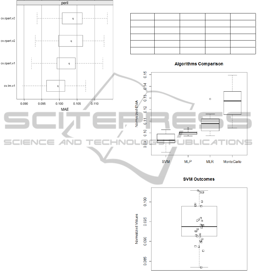
Figure 5: Boxplots for normalized errors of linear regres-
sion models.
standard deviation (Std.) value.
In Figure 6, it is observed that the traditional tech-
nique, MCS (monte carlo simulation), had a large
standard deviation. It is due to randomness in MCS
method, one of its limitation. Besides that, MCS had
higher statistics. On the other hand, comparing MCS
with MLR it is noticed that MLR had better statistics.
Thus, for this study, we could not identify a reason
to justify MCS usage for risk analysis, proposed by
(Institute, 2008). That was one of our premises.
Besides that, MLP seemed to be a promising al-
ternative because it is like a optimized MLR, because
MLP is a universal approximator of nonlinear func-
tions and its efficiency was proven in the most differ-
ent application areas. In this study, MLP was a more
precise method to risk impact estimation.
Commonly, SVM has a higher generalization ca-
pability, which means 1.5% better results compared
with MLP, approximately (Haykin, 1994). That is be-
cause SVM can distinguish small subsets in training
data. However, it requires a long training time due to
its complexity.
Therefore, accordingly with this study, SVM
seems to be a more accurate method to risk impact es-
timation using PERIL. We can conclude that because
it explored a lesser MAE and had a good generaliza-
tion capability, since its inter-quartil interval was the
second shorter, according to Figure 6. But above all,
SVM could explore MAE optimization problem. We
can realize it observing Figure 7, in which the most of
values are near and above median value.
Table 4: Descriptive statistics for SVM, MLP, MLR and
MCS.
SVM MLP MLR MCS
Min. 0.08347 0.09736 0.09764 0.10410
Median 0.09374 0.10014 0.10798 0.12740
Mean 0.09430 0.10005 0.10798 0.12640
Std. 0.00488 0.00154 0.00794 0.01250
Max. 0.10284 0.10413 0.12927 0.14950
Figure 6: Boxplots of analyzed methods.
Figure 7: SVM boxplot with individual values.
5 CONCLUSION
This paper has investigated the use of artificial neu-
ral networks algorithms, like SVM and MLP, for es-
timation of risk impact in software project risk analy-
sis. We have carried out a statistical analysis using
PERIL. The results were compared to MLRM and
Monte Carlo Simulation, a traditional approach pro-
posed by (Institute, 2008). We have considered im-
ICEIS2014-16thInternationalConferenceonEnterpriseInformationSystems
478

proving risk impact estimation accuracy during soft-
ware project management, in terms of MAE mean
and standard deviation. We have observed that MLP
had minor standard deviation estimation error, and
showed to be a promissory technique. Moreover,
SVM had minor estimation error outcomes using
PERIL, which a more accurate method. Therefore,
the selected ANN algorithms outperformed both lin-
ear regression and MCS. Future works should analyze
another ANN models and MLP training methods.
REFERENCES
Amari, S., Murata, N., M
¨
uller, K.-R., Finke, M., and Yang,
H. (1996a). Statistical theory of overtraining-is cross-
validation asymptotically effective? Advances in neu-
ral information processing systems, pages 176–182.
Amari, S.-i., Cichocki, A., Yang, H. H., et al. (1996b).
A new learning algorithm for blind signal separation.
Advances in neural information processing systems,
pages 757–763.
Attarzadeh, I. and Ow, S. H. (2010). A novel soft com-
puting model to increase the accuracy of software
development cost estimation. In Computer and Au-
tomation Engineering (ICCAE), 2010 The 2nd Inter-
national Conference on, volume 3, pages 603–607.
IEEE.
Bannerman, P. L. (2008). Risk and risk management in soft-
ware projects: A reassessment. Journal of Systems
and Software, 81(12):2118–2133.
Boehm, B. W. (1991). Software risk management: principle
and practices. IEEE Software, 8:32–41.
Budzier, A. and Flyvbjerg, B. (2013). Double
whammy-how ict projects are fooled by random-
ness and screwed by political intent. arXiv preprint
arXiv:1304.4590.
Dan, Z. (2013). Improving the accuracy in software ef-
fort estimation: Using artificial neural network model
based on particle swarm optimization. In Service Op-
erations and Logistics, and Informatics (SOLI), 2013
IEEE International Conference on, pages 180–185.
IEEE.
Dzega, D. and Pietruszkiewicz, W. (2010). Classification
and metaclassification in large scale data mining ap-
plication for estimation of software projects. In Cy-
bernetic Intelligent Systems (CIS), 2010 IEEE 9th In-
ternational Conference on, pages 1–6. IEEE.
Haimes, Y. Y. (2011). Risk modeling, assessment, and man-
agement. John Wiley & Sons.
Hall, M., Frank, E., Holmes, G., Pfahringer, B., Reutemann,
P., and Witten, I. H. (2009). The weka data min-
ing software: an update. ACM SIGKDD Explorations
Newsletter, 11(1):10–18.
Han, J., Kamber, M., and Pei, J. (2006). Data mining: con-
cepts and techniques. Morgan kaufmann.
Haykin, S. (1994). Neural networks: a comprehensive foun-
dation. Prentice Hall PTR.
Higuera, R. P. and Haimes, Y. Y. (1996). Software risk man-
agement. Technical report, DTIC Document.
Hu, Y., Huang, J., Chen, J., Liu, M., and Xie, K. (2007).
Software project risk management modeling with neu-
ral network and support vector machine approaches.
In Natural Computation, 2007. ICNC 2007. Third In-
ternational Conference on, volume 3, pages 358–362.
IEEE.
Huang, X., Ho, D., Ren, J., and Capretz, L. F. (2004). A
neuro-fuzzy tool for software estimation. In Software
Maintenance, 2004. Proceedings. 20th IEEE Interna-
tional Conference on, page 520. IEEE.
Institute, P. M. (2008). A Guide to the Project Management
Body of Knowledge.
Kendrick, T. (2003). Identifying and managing project risk:
essential tools for failure-proofing your project. Ama-
com: New York.
Kwak, Y. H. and Ingall, L. (2007). Exploring monte carlo
simulation applications for project management. Risk
Management, 9(1):44–57.
Priddy, K. L. and Keller, P. E. (2005). Artificial Neural
Networks: An introduction, volume 68. SPIE Press.
Rumelhart, D. E., Hinton, G. E., and Williams, R. J. (1985).
Learning internal representations by error propaga-
tion. Technical report, DTIC Document.
Saxena, U. R. and Singh, S. (2012). Software effort esti-
mation using neuro-fuzzy approach. In Software En-
gineering (CONSEG), 2012 CSI Sixth International
Conference on, pages 1–6. IEEE.
Schmidt, R., Lyytinen, K., Keil, M., and Cule, P. (2001).
Identifying software project risks: an international
delphi study. Journal of management information sys-
tems, 17(4):5–36.
Shevade, S., Keerthi, S., Bhattacharyya, C., and Murthy, K.
(1999). Improvements to the smo algorithm for svm
regression. In IEEE Transactions on Neural Networks.
Siegel, S. (1956). Nonparametric statistics for the behav-
ioral sciences.
Smola, A. and Schoelkopf, B. (1998). A tutorial on support
vector regression. Technical report. NeuroCOLT2
Technical Report NC2-TR-1998-030.
Support, I. P. (2005). Monte Carlo Simulation. Ibbot-
sonAssociates, 225 North Michigan Avenue Suite 700
Chicago, IL 60601-7676.
Taleb, N. (2001). Fooled by randomness. Nwe York: Ran-
dom House.
Torgo, L. (2003). Data mining with r. Learning by
case studies. University of Porto, LIACC-FEP. URL:
http://www. liacc. up. pt/ltorgo/DataMiningWithR/.
Accessed on, 7(09).
Valenca, M. J. S. (2005). Aplicando redes neurais: um guia
completo. Livro Rapido, Olinda–PE.
Venables, W. N., Smith, D. M., and Team, R. D. C. (2002).
An introduction to r.
Yu, P. (2011). Software project risk assessment model based
on fuzzy theory. Computer Knowledge and Technol-
ogy, 16:049.
EvaluatingArtificialNeuralNetworksandTraditionalApproachesforRiskAnalysisinSoftwareProjectManagement-A
CaseStudywithPERILDataset
479
