Multi-objective Optimization of Investment Strategies

Based on Evolutionary Computation Techniques, in Volatile Environments

Jose Matias Pinto, Rui Ferreira Neves and Nuno Horta

Instituto de Telecomunicações, Instituto Superior Técnico, Torre Norte, Piso 10, Lisboa, Portugal

Keywords: Multi-objective Optimization, Stock Market Forecast, Technical Analysis, Financial Markets, Moving

Average, Time Series Prediction.

Abstract: In this document, the use of a multi-objective evolutionary system to optimize an investment strategy based

on the use of Moving Averages is proposed to be used on stock markets, able to yield high returns at

minimal risk. Fair and established metrics are used to both evaluate the return and the risk of the optimized

strategies. The Pareto Fronts obtained with the training data during the experiments conducted outperform

both B&H strategy and the classical approaches that consider solely the absolute return. Additionally, the

PF obtained show the inherent trade-off between risk and returns. The experimental results are evaluated

using data coming from the principal world markets, namely, the main stock indexes of the most developed

economies, such as: NASDAQ, S&P500, FTSE100, DAX30 and NIKKEI225. Although, the experimental

results suggest that the positive connection between the gains with training and testing data, usually

assumed in the single-objective proposals, is not necessarily true for all cases.

1 INTRODUCTION

Besides some unfavourable judgments (Korczak et

al., 2002), Technical Indicators (TI) are still widely

used as tools to do the technical analysis of financial

markets, exploiting the existence of trends to

establish potential buy, sell or hold conditions. This

study is notoriously tricky for a number of reasons,

though (Achelis, 2000) has made a complete

reference that fully explains the most important TI's

one can identify and use. Anyway, the main

difficulty of TI usage is still deciding its suitable

parameter values, as number of days of periods, and

this, in order to take advantage of the market and

improve your likelihood of success.

Thus, evolutionary computation appears as a

highly suitable alternative to extend technical

analysis of financial markets to tune the parameters

of some chosen TI (or set of TI's), so that, the

desired goals are achieved, at maximum extent

possible. In this environment, what the system

should do, can be viewed as some kind of predicting

future stock prices. Consequently, in this context,

evolutionary computation emerges as a stochastic

search technique able to deal with highly

complicated and non-linear search spaces.

In the last decade, several financial crises have

occurred with large consequences on the valorisation

of financial assets. Therefore emerges the principal

motivation for this paper: tune an Investment or

Trading Strategy (TS) able to achieve both the

highest returns with the minimal risk.

One of the goals of this work is to tune a TS to

present the highest returns as existing single

objective based approaches, and concurrently reduce

the risk. The proposed framework is tested using

data from the main stock indexes of the most

developed economies, such as NASDAQ, S&P500,

FTSE100, DAX30 and NIKKEI225; then the results

are presented, and some possible conclusions

outlined.

The next section will present the related work

using GA and the various TS's currently used in

Technical Analyses. In Section 3 the methodology,

the roles of the most relevant modules used to build

the proposed framework, and the chromosome

encoding are outlined. The TS adopted in this study

and the metrics used to evaluate the evolved TS are

also presented in this section. Section 4 presents the

results and the most relevant outcomes are

highlighted. Finally, in section five, the conclusions

of this study are presented.

480

Matias Pinto J., Ferreira Neves R. and Horta N..

Multi-objective Optimization of Investment Strategies - Based on Evolutionary Computation Techniques, in Volatile Environments.

DOI: 10.5220/0004889204800488

In Proceedings of the 16th International Conference on Enterprise Information Systems (ICEIS-2014), pages 480-488

ISBN: 978-989-758-027-7

 2014 SCITEPRESS (Science and Technology Publications, Lda.)

2 RELATED WORK

Stock market analysis has been one of the most

attractive and active research fields, where many

Machine Learning techniques have been used.

Generally speaking, one can distinguish two

methods for anticipating future stock prices and the

time to buy or sell; one is Technical Analysis

(Murphy, 1999) and the other is Fundamental

Analysis (Graham et al., 2003). Fundamental

Analysis look at stock prices using financial

statement of each company, economic trend and so

on; requires a large set of financial and accounting

data, difficult to obtain and both released with some

delay and often suffers of low consistency.

Technical Analysis numerically analyzes the past

movement of stock prices, is based on the use of

technical stock market indicators that work on a

series of data, usually stock prices or volume,

(Achelis, 2000) is accurate, on time, and relativity

easy to obtain. Consequently, this work will be

focused on the use of Technical Analysis to

anticipate future stock price movements.

Many approaches based on evolutionary

computation have been proposed and applied to

diverse fields of financial to predict worth trends. In

an attempt to summarize, in most of the works, the

generated returns are exclusively used as the only

fitness metric, without accounting for the related

risk. Some examples are the use of GAs to optimize

TI's parameters (Fernández-Blanco et al., 2008), or

to develop TS based on TI's (Bodas-Sagi et al.,

2009), (Gorgulho et al., 2011).

According to what was stated for the first time in

1952 (Markowitz, 1952), any TS should have the

highest possible profit with the feasible minimal

risk. Sadly, these two metrics are intrinsically

conflicting by virtue of the risk-returns trade-off.

Some articles propose the combination of the two

conflicting objectives into one single metric, in

particular (Bodas-Sagi & al., 2009) use the Chicago

Board Options Exchange (CBOE) Volatility Index

(VIX) as an estimate of risk. Also, (Schoreels & al.,

2006) propose the use of a Capital Asset Pricing

Model (CAPM) (William, 1964) system, based on

portfolio theory (Markowitz, 1952) to reduce risk

trough balanced selection of securities. More

recently (Pinto et al., 2011) propose and study

several alternatives to the classical fitness evaluation

functions.

A Multi-Objective system to maximize the total

returns and to minimize the risk as the exposure to it

is proposed by (Chiam et al., 2009). The framework

is tested using data gotten from one stock market,

the Singapore Exchange stock market (Straits Times

Index (STI)). Hence, some of the conclusions drawn

on this study could be attributed to the market used

to test it. Moreover, the metric used to evaluate the

return is peculiarly unusual; so, it is difficult, to

compare the presented results with the results

presented by other alternative applications.

3 METHODOLOGY

The proposed system consists of a Multi Objective

Genetic Algorithm coupled with a market return

evaluation module that does the fitness evaluation,

and this, based on the estimation of the two

conflicting objectives, on the chosen market, and on

the specified period.

3.1 Strategy and Parameters

The strategy tested on this work was the Moving

Average Crossover (MAC), which is based on the

use of two Moving Averages (MA), with different

periods. One, formed by the MA with the shorter of

the two periods is called the "Fast MA”, and the

other, with the longer period is the "Slow MA". The

"Fast MA" reflects changes earlier than does the

"Slow MA". A buying (or sell short) signal is

generated when the Fast MA crosses over the Slow

MA. Conversely, sell (or a buy short) signal is

generated when the Fast MA crosses under the Slow

MA.

After defining the strategy, it is necessary to

define the parameters of the MAC, which in the case

are the type of the MA’s and the corresponding

period. It is important to stress that, for the type of

MA to use, the GA has also the freedom to choose

between a Simple or an Exponential MA.

Although it is common to tune the parameters of

one single TI and then use it to generate buy and sell

signals, for both long and short positions, in this

article, the option of using a separate set of

parameters for each of the possible actions was

taken; to specify: "enter long"; "exit long"; "enter

short"; and "exit short".

Some pre-processing of the historical data is also

done. This applies for instance to the MA periods,

which are calculated at program start and are limited

to the following set of Simple or Exponential MA's:

1, 4, 8, 12, 14, 16, 20, 24, 28, 32, 36, 40, 55, 60, 65,

70, 75, 80, 85, 90, 95, 100, 110, 120, 130, 140, 150,

160, 170, 180, 190, 200 and 250 days. This set of

periods has been chosen because it covers the most

widely used, long and short-term MA periods, found

Multi-objectiveOptimizationofInvestmentStrategies-BasedonEvolutionaryComputationTechniques,inVolatile

Environments

481

on books and recommended by experts (Achelis,

2000).

3.2 Genetic Encoding

The chromosome must represent the MAC indicator

used, this way one MAC chromosome is represented

by two genes: one represents the type and the period

of the Fast MA and the other does the same for the

Slow. These entries are natural numbers in the

interval of values between 0 and 65 as it encodes, in

one single entry (integer variable) the type of MA

and its period. In Table 1 is represented the

chromosome structure.

Table 1: Chromosome representation.

Parameters

Enter long

position

Exit long

position

Exit short

position

Enter short

position

Fast

Slow

Fast

Slow

Fast

Slow

Fast

Slow

Chromosome

0..65 0..65 0..65 0..65 0..65 0..65 0..65 0..65

3.3 Fitness Evaluation

The fitness evaluation process is concerned with

simulating the performance of the each trading agent

in the evolving population and calculating the

corresponding total returns and the related risk. The

resultant fitness values of the trading agent must be

evaluated under some established and fair metric, as

will be discussed in the next subsections.

3.3.1 Return Metric

The profits generated by a given TS can be

measured in different ways, as will be seen next:

For instance, the potential profits can be estimated

by simply summing the area under the total asset

graph during the trading period (Schoreels et al.,

2005). Alternatively, another return metric could be

the final (total) assets; this means the available

capital plus the value of all holdings, at the end of

the investment period (Kendall et al., 2003). Sadly,

both above metrics have the nuisance that they are

always attached to the initial cash invested.

Therefore, an alternative metrics exists that

considers its relative value and is known as Return

on Investment (ROI),. This metric is a ratio and

represents the money gained or lost on an

investment relative to the amount of money

invested. ROI is usually expressed as a percentage,

and for one period, by definition, is calculated

according with equation 1. “Profit” is the amount of

money gained or lost and “Initial_Investment” is the

money invested.

Profit

ROI

Initial Investiment

inal_Assets Initial_Investiment

Initial Investiment

Final_Assets

Initial Investiment









(1)

ROI still has the trouble that, for multi-period

investment, it is difficult to compare it with the

results one would get in one single period.

Therefore, a metric that could be compared with

similar alternative investments should be used

instead. This way, in this article, the Annualized

ROI, will be used. The Annualized ROI is nothing

more than the “Geometric Average of the Ratio of

the Returns” also known as the "True Time-

Weighted Rate of Returns". Mathematically, for an

investment lasting for N periods, with full

reinvestment, is computed as exposed in equation 2;

in this equation, N is the number of periods, more

exactly, the number of years, the investment lasts.

() ( 1)1

Anualised ROI ROI





(2)

3.3.2 Risk Metrics

Risk is usually seen as the volatility or the

uncertainty of the expected returns over the

investment period. Therefore, the linked risk of any

investment technique can be estimated in several

ways, as will be examined subsequently.

The most traditional risk metric is inherited from

statistics and from Markowitz Mean-Variance

Model (Markowitz, 1952), and consists in the use of

the variance of the results as a gauge for the risk.

This variance can be calculated using the standard

deviation or the variance between the returns, this

statistical measure of the dispersion of the results is

usually named, in finance, as volatility.

Instead, risk can be computed as the exposure to

it (Weissman, 2005). Specifically, it can be

measured by the proportion of trading days when a

position is maintained open on the market, and is,

mathematically, the ratio between the time the agent

is on the market and the total trading time available.

Essentially, staying longer in the market corresponds

to a higher exposure to risk, like market crashes and

other disastrous events, while shorter periods on the

market correspond to a lower risk exposure and

greater liquidity (as the capital is engaged for a

smaller time).

Alternative metrics for the risk can be found on

the literature, as, for instance, the use of some risk-

adjusted return metric, as the Sharpe ratio, Sortino

ratio, Sterling ratio (SR), Calmar ratio (CR) or also

ICEIS2014-16thInternationalConferenceonEnterpriseInformationSystems

482

VIX which compute the net profitability after

discounting the associated risk (Korczak et al.,

2004). In short, the preceding risk metrics are in

reality alternative methods to combine into one

single objective (or metric) the two conflicting

objectives faced on this kind of problems (risk and

return).

Therefore, in the remaining of this paper, the risk

exposure will be used as the risk metric.

3.4 Optimisation Kernel

This study is concerned with the Evolutionary

Optimization of a TS treated as a multi-objective

problem, so the Optimisation Kernel is based on a

version of a state of the art multi-objective

evolutionary algorithm: Non Dominated Sorting

Genetic Algorithm 2 (NSGAII) (Deb et al, 2002).

NSGAII parameters are as follows: population size

500, the crossover probability fixed to 0.8 and

parents selected by tournament selection. Each run

on training data continued for 300 generations and

the probability of real mutation set to 0.1.

3.5 The Investment Simulator

The Investment Simulator or Market Return

Evaluation Module simulates an investment in the

user specified index including long and short

positions. Stock market index, which it could buy

(“go long”), sell it and stay out of the market (“Out”)

or even sell if it didn’t own any (“go short”) hoping

to profit from a decline in the price of the assets

between the sale and the repurchase.

Since daily data was available, the training

consisted in formulating an TS, give to the agent

some initial cash to spend, and every day simulate

the performance of the agent; having it to buy or sell

(“long” or “short”) the total cash available, if the

conditions defined on its encoded strategy are met.

Transaction costs were not included in the

simulation, as dividends not too. Environment is also

assumed discrete and deterministic in a liquid

market.

4 RESULTS

A multi-objective evolutionary optimization of a TS

is studied in this essay what involves the

maximization of a Return Metric and the

minimization of the related Risk Metric. In this kind

of problems the optimal solutions exist in the form

of a set of tradeoffs known as the Pareto-optimal set

(PF); and any objective belonging to a solution in

the optimal set cannot be improved without

degrading at least one of the others objectives.

An example of a possible PF is illustrated in

Figure 1, and this represents clearly the risk-return

trade-off or Efficient Frontier always faced in this

kind of problems.

Figure 1: Risk Return Trade-off.

On this illustration, each point denotes a Strategy

evolved by the GA. The black circles and the white

crosses represent non-dominated and dominated

solutions respectively. The set formed by the former

solutions is the Pareto optimal solution set because

their returns cannot be improved further without

compromising risk. In the context of single objective

optimization where return is the only goal, the

evolutionary process will ultimately drive the

solutions towards the extreme point B. This is not

applicable to conservative investors, who may prefer

a lower risk at a cost of lower returns. Point A

represents the extreme case of a conservative

investor with zero returns due to his total risk

adversity.

4.1 Training and Testing Data Sets

The system was tested using historical daily prices

from the stock indexes: S&P 500, FTSE 100, DAX

30, NIKKEI 225 and NASDAQ.

The period of time chosen for training was from

3 Jan. 2000 to 31 Dec. 2007. This time period was

assumed sufficient to evolve a competitive

population as it exhibited significant movement,

including several boom and crash periods. For out of

sample and testing period, two years of data was

used, and it was from 2 Jan. 2008 to 31 Dec. 2009.

Multi-objectiveOptimizationofInvestmentStrategies-BasedonEvolutionaryComputationTechniques,inVolatile

Environments

483

4.2 Analysis of the Training

Performance

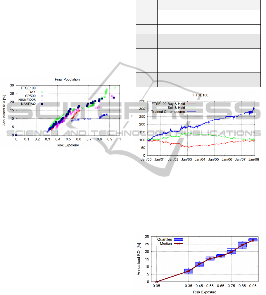
Figure 2 present the PF's evolved for the 5 indexes

tested in this study, in one of the experimental runs

performed. Though the various solutions sets vary in

terms of Pareto dominance and optimality, all

clearly illustrate the inherent trade-off between

return and risk. Furthermore, the trading agents

evolved are able to generate high returns in open

positions less than 100% of the trading period, for

instance, the observable annualized ROI near or

above 10% with risk exposure around 0.6.

Figure 2: Evolved Pareto Fronts for the five Indexes

Tested.

In Financial Computing when analyzing the

performance of a given TS, it is common to compare

it against the “Buy & Hold” (B&H) and “Sell &

Hold” (S&H) strategies. When the ROI performance

of the evolved TS (see figure 2) is compared against

both B&H and S&H approaches (see B&H and S&H

annualised ROI calculation on Table 2), during the

training period, it is easy to conclude that, in this

context, both B&H and S&H strategies are

undoubtedly suboptimal. It is also important to

remind that both, B&H and S&H, strategies

correspond to a risk exposure of 1 (one); since the

capital is all time engaged.

In Figure 3 is presented an example of the eight-

year financial data used to optimize the strategy, in

the current case is the FTSE100 index. The line

labelled “Buy & Hold” characterizes the

performance of the B&H strategy; this same line is

coincident with the current index evaluation at close

price. On this same illustration, the performance of

the S&H strategy is exposed by the curve tagged

“Sell & Hold”. An example of the trading

performance of one of the optimized strategies is

also shown on this figure, by the line labelled

“Trained Chromosome”. On the same illustration the

X axis is the time, and on the Y axis is the assets

evaluation.

Table 2: Annualized ROI for B&H and S&H strategies in

the training period.

NIKKEI

225

FTSE

100

S&P500 DAX30 NASDAQ

B&H

Absolute

Return

-3695.08 - 206.00 13.14 1316.56 -1478.87

B&H ROI

[%]

- 19.44% - 3.09% 0.90% 19.50% - 35.80%

B&H

Annualized

ROI [%]

-2.67% -0.39% 0.11% 2.25% -5.39%

S&H

Absolute

Return

3695.08 206.00 -13.14 -1316.56 1478.87

S&H ROI

[%]

19.44% 3.09% - 0.90% - 19.50% 35.80%

S&H

Annualized

ROI [%]

2.25% 0.38% -0.11% -2.67% 3.90%

Figure 3: Example of daily closing prices and the

performance of one trained agent, for FTSE100 index, in

the training period.

In order to have a better insight about the data and

results, 30 (thirty) experimental runs were

performed, the results collected, and then, discrete

intervals of 0.1 of risk exposure considered. With

this data, plots like the one shown in Figure 4 were

gotten.

Figure 4: Annualised ROI in discrete intervals of 0.1 Risk

Exposure, observed with DAX index.

Figure 4 plots an example of the observed

distribution of the Annualized ROI in function of the

risk exposure. This illustration shows the First

Quartile of data (Q1), the Third Quartile of data

(Q3), as well the Median, with the whiskers located

ICEIS2014-16thInternationalConferenceonEnterpriseInformationSystems

484

respectively at 10% and 90% of data, and this for the

results observed, with training data. Again, the risk-

returns trade-off is evident, since the average of the

Annualized ROI increases for higher levels of risk

exposure. The lack of solutions in the risk exposure

range of 0.1 to 0.2 can be due to the difficulty in

optimizing the chosen TI to exploit the price

movements in order to create strategies in this

region. Similar plots, identical the one shown, were

also observed for the further indexes also tested in

this study.

4.3 Correlation Analysis of Training

and Testing Performance

The results presented in the previous subsection

showed that it is possible to tune a TS to attain

attractive returns at various levels of risk exposure.

Despite this, the great effectiveness of any approach

will depend on being able to extend these interesting

returns to unseen data, which is usually recognized

as its generalization performance.

In order to evaluate the engine generalization

performance, the available trading data is portioned

into two independent sets of data, this means:

training and testing data sets, as explained in

subsection 4.1. In the training phase of the

evolutionary process, the TS will be trained, tuned

and evaluated using only training data. After being

trained, the developed strategies obtained in the final

generation will be then applied to the testing data set

and its generalization performance is evaluated. This

is an indicator of the framework real effectiveness in

getting good results using unseen data.

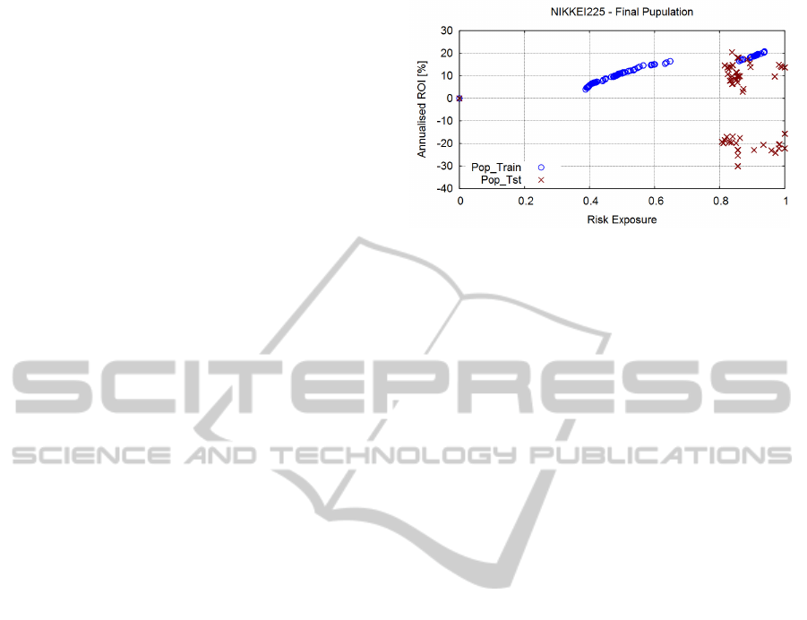
The plot of the risk-returns PF's for the training

data gotten in one of the experimental run is

presented in Figure 5. The marks labelled

“Pop_Train” represent the final population evolved

after 400 generations, while the points tagged

“Pop_Tst” represent the results of this same

population when applied to the testing data set.

The example shown on Figure 5 is for the

NIKKEI index, but similar plots were observed with

the further indexes also tested.

Again, in this plot, the risk-returns trade-off is

evident with the training data. However, such

correlation disappears when the same strategy is

applied to the testing data. For instance, annualized

ROI of 15% are realizable at a risk level of 0.6 with

the training data, while big losses are gotten at the

same level of risk with the testing data. This low

relation between training and testing results was also

observed in previous studies (Korczak et al., 2004),

(Chiam et al, 2009).

Figure 5: Pareto Fronts observed with training and testing

data.

The most evident conclusion from this figure is that

positive returns with the training data do not

necessarily match to positive returns with the testing

data.

Hence, it urges the need to better understand

how the training and testing data correlate together,

in order to examine the generalization performance

of the evolved TS's. This suggests that a correlation

analysis between the four variables involved should

be conducted; to name: training ROI, training risk,

testing ROI and testing risk.

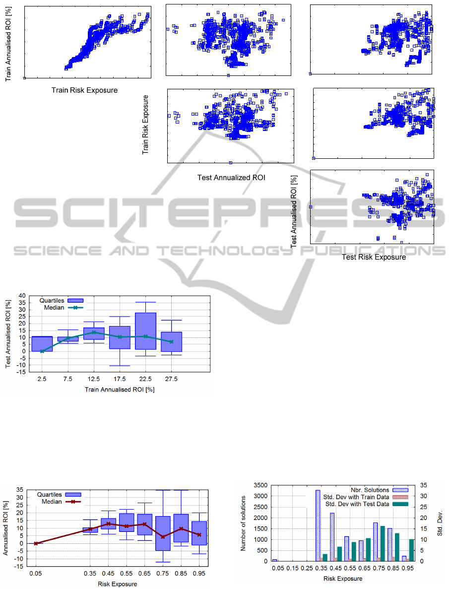
To better clarify the results, 30 independent

experimental runs were performed and with the

results observed in these experimental runs, the

graphs shown in Figure 6 where build. On this

graphs the variables are plotted and its potential

correlations can be visually inspected. Once more,

the plot of training ROI and training risk accurately

shows the risk-returns trade-off. While an almost

random plot is obtained when the testing returns

against the testing risk are plotted, therefore this

suggests the existence of low correlation between

training ROI and testing ROI.

Contrasting to the traditional theory in single-

objective approaches where higher training returns

are coupled with higher testing returns, this

relationship is missing from these plots. Instead,

higher training returns correspond to increased

volatility in the observed testing returns; this is

clearly observable in the graph of Figure 7. This

figure plots the quartiles of data (Q1-Q3), the

median, as well the whiskers located respectively at

10 and 90% of the observed results, when the

training returns are divided in discrete intervals of

5%. On this figure the median of the testing returns

does not boost when the values of training returns

increase. In its place, there is a visible increase in the

variance of the results, denoted by largest vertical

lines (both whiskers and boxes).

Multi-objectiveOptimizationofInvestmentStrategies-BasedonEvolutionaryComputationTechniques,inVolatile

Environments

485

0 0.2 0.4 0.6 0.8 1

Train Annualized ROI [%]

Test Time on Market

-0.4 -0.3 -0.2 -0.1 0 0.1 0.2 0.3 0.4

Train Annualized ROI [%]

Test Annualized ROI

0 0.1 0.2 0.3 0.4 0.5 0.6 0.7 0.8 0.9 1

Train Annualized ROI [%]

Train Time on Market

0.1

0.2

0.3

0.4

0.5

0.6

0.7

0.8

0.9

0 0.2 0.4 0.6 0.8 1

Train Time on Market

Test Time on Market

-40

-30

-20

-10

0 0.2 0.4 0.6 0.8 1

Test Annualized ROI [%]

Test Time on Market

0.1

0.2

0.3

0.4

0.5

0.6

0.7

0.8

0.9

-0.4 -0.3 -0.2 -0.1 0 0.1 0.2 0.3 0.4

Train Time on Market

Test Annualized ROI

Figure 6: Plots showing the correlation between training returns, training risk, testing returns and testing risk.

Figure 7: Statistical distribution of testing returns at

discrete intervals of the training returns for DAX index.

In conclusion, the positive correlation typically

implicit in conventional single-objective approaches,

to do the optimization of TS's, between training and

testing returns, is not necessarily true for all cases.

Figure 8: Distribution of testing returns at discrete

intervals of training risk for DAX index.

Similar conclusions can be extracted from the

plot shown in Figure 8 where the testing returns

observed in the 30 independent runs are resumed at

discrete intervals of 0.1 training risk. Again, the

median of the testing returns does not increase when

the training risk increases.

Although, a steady increase is clearly observable

in the variance of the test returns is clear from the

plots (Figures 8 and 9), what confirms the claim that

higher training returns correspond to increased

volatility in the test returns results.

Figure 9 shows the number of solutions gotten in

each interval of test risk exposure (scale at left)

together with the Std. Dev. gotten with both the

training data and testing data (scale at right). The

apparent drop in the test results volatility for risk

Figure 9: Number of Solutions and Standard deviation of

the testing returns at discrete intervals of 0.1 risk exposure

for DAX Index.

ICEIS2014-16thInternationalConferenceonEnterpriseInformationSystems

486

level above 0.8 is statistically irrelevant as there are

few solutions in this region. The plots presented

were built with the DAX results, but similar plots

were also observed for the remaining four indexes

also tested in this study.

4 CONCLUSIONS

This document presented and investigated a multi-

objective evolutionary approach to do the

optimization of a set of TS’s. In this work, fair and

established metrics were used to both evaluate the

return and the related risk. Both metrics were

simultaneously optimized and a popular TI

frequently used by real-world professionals was

used as the building block of the core strategy.

Furthermore, the TS’s were trained, and afterwards

tested, using data coming from five main stock

indexes, representative of the world most developed

economies. The PF’s obtained by the algorithm

using testing data correctly depict the intrinsic trade-

off between risk and return.

The low correlation between training returns and

testing returns conducted to deceptive results when

the testing results are analyzed, what suggests a low

potential in the framework generalization capability.

Consequently, the experimental results suggest that

the positive connection between training and testing

returns usually assumed in conventional single-

objective approaches may not necessarily hold true

for all cases.

Anyway, some interesting conclusions can be

extracted, namely the conclusion that higher training

returns correspond to increased volatility in the

testing results. The MAs have the disadvantage of

being a trend follower indicator, so the signals one

can get from such indicator are always with some

delay. Further tests should be accomplished, using

other TI and the achieved results should be seen as a

benchmark to further improvements with the use of

other TI, or even the use of multi TI strategies.

REFERENCES

Achelis, S. B., 2000. Technical Analysis from A to Z, 2nd

Edition, McGraw-Hill, New York, 2nd Edition, New

York, (October 2, 2000).

Bodas-Sagi, Diego J., Fernández, Pablo, Hidalgo, J.

Ignacio, Soltero, Francisco J., Risco-Martín, José L.,

2009. Multiobjective Optimization of Technical

Market Indicators. In Proceedings of the 11th Annual

Conference Genetic and Evolutionary Computation

Conference (GECCO). Montreal, Canada, 1999–2004.

Chiam, Swee Chiang, Tan, Kay Chen, Mamun, Abdullah

Al, 2009. Investigating technical trading strategy via

an multi-objective evolutionary platform. In Expert

Systems with Applications. 36, 7, (Sep., 2009), 10408-

10423.

Deb, Kalyanmoy, Pratap, Amrit, Agrawal, Samir,

Meyarivan, T., 2002. A fast and elitist multi-objective

genetic algorithm: NSGA-II. In IEEE Transactions on

Evolutionary Computation. IEEE Computer Society,

Washington, DC, USA, 6, 2, (Apr, 2002), 182-197.

Fernández-Blanco, Pablo, Bodas-Sagi, Diego J., Soltero,

Francisco J., Hidalgo, J. Ignacio, 2008. Technical

Market Indicators Optimization Using Evolutionary

Algorithms. In Proceedings of the 2008 GECCO

conference on Genetic and evolutionary computation

(GECCO). Atlanta, Georgia. USA, 1851-1857.

Gorgulho, António, Neves, Rui, Horta, Nuno, 2011.

Applying a GA kernel on optimizing technical

analysis rules for stock picking and portfolio

composition. In Expert Systems with Applications

(ESWA). 38, 11, (October 2011), 14072–14085.

Graham, Benjamin, Zweig, Jason, Buffett, Warren E.,

2003. The Intelligent Investor, Revised edition, Collins

Business, Revised edition, (July 8, 2003).

Kendall, Graham, Su, Yan, 2003. A multi-agent Based

Simulated Stock Market – Testing on Different Types

of Stocks. In Proceedings of the 2003 Congress on

Evolutionary Computation (CEC’03). 4, 2298-2305.

Korczak, J.J., Lipinski, Piotr, 2004. Evolutionary Building

of Stock Trading Experts in a Real-Time System. In

Proceedings of the 2004 Congress on Evolutionary

Computation (CEC 2004). Portland, USA, (19-23

June, 2004), 940-947.

Korczak, Jerzy, Roger, Patrick, 2002. Stock Timing Using

Genetic Algorithms in Applied Stochastic models. In

Business and Industry. 18, (January 15, 2002), 121-

134.

Markowitz, Harry M., 1952. Portfolio Selection. In The

Journal of Finance. 7, 1, (Mar., 1952), 77-91.

Murphy, John J., 1999. Technical Analysis of Financial

Markets, Prentice Hall Press, New York Institute of

Multi-objectiveOptimizationofInvestmentStrategies-BasedonEvolutionaryComputationTechniques,inVolatile

Environments

487

Finance, New York. (January 4, 1999).

Pinto, J., Neves, R. F., Horta, N., 2011. Fitness function

evaluation for MA trading strategies based on genetic

algorithms. In Proceedings of the 13th annual

conference companion on Genetic and evolutionary

computation (GECCO '11). ACM, New York, NY,

USA, 819-820.

Schoreels, Cyril, Garibaldi, Jonathan M., 2005. A

comparison of adaptive and static agents in equity

market trading. In Proceedings of the EEE/WIC/ACM

International Conference on Intelligent Agent

Technology (IAT '05). Compiegne, France, 393-399.

Schoreels, Cyril, Garibaldi, Jonathan M., 2006. Genetic

algorithm evolved agent-based equity trading using

Technical Analysis and the Capital Asset Pricing

Model. In Proceedings of the 6th International

Conference on Recent Advances in Soft Computing

(RASC2006). Canterbury, UK, 194-199.

Weissman, Richard L., 2005. Mechanical Trading

Systems: Pairing Trader Psychology with Technical

Analysis, Wiley Trading. Wiley Trading.

William, F. Sharpe, 1964. Capital Asset Prices: A Theory

of Market Equilibrium under Conditions of Risk. In

The Journal of Finance. 19, 3, (Sep., 1964), Blackwell

Publishing, American Finance Association, 425-442.

ICEIS2014-16thInternationalConferenceonEnterpriseInformationSystems

488