
Efficient and Distributed DBScan Algorithm Using MapReduce
to Detect Density Areas on Traffic Data
Ticiana L. Coelho da Silva, Ant
ˆ
onio C. Ara
´
ujo Neto, Regis Pires Magalh
˜
aes, Victor A. E. de Farias,
Jos
´
e A. F. de Mac
ˆ
edo and Javam C. Machado
Federal University of Ceara, Computing Science Department, Fortaleza, Brazil
Keywords:
DBScan, MapReduce, Traffic Data.
Abstract:
Mobility data has been fostered by the widespread diffusion of wireless technologies. This data opens new
opportunities for discovering the hidden patterns and models that characterise the human mobility behaviour.
However, due to the huge size of generated mobility data and the complexity of mobility analysis, new scalable
algorithms for efficiently processing such data are needed. In this paper we are particularly interested in using
traffic data for finding congested areas within a city. To this end we developed a new distributed and efficient
strategy of the DBScan algorithm that uses MapReduce to detect what are the density areas. We conducted
experiments using real traffic data of a brazilian city (Fortaleza) and compare our approach with centralized
and map-reduce based DBSCAN approaches. Our preliminaries results confirm that our approach is scalable
and more efficient than others competitors.
1 INTRODUCTION
Mobility data has been fostered by the widespread
diffusion of wireless technologies, such as the call de-
tail records from mobile phones and the GPS tracks
from navigation devices, society-wide proxies of hu-
man mobile activities. These data opens new opportu-
nities for discovering the hidden patterns and models
that characterize the trajectories humans follow dur-
ing their daily activity. This research topic has re-
cently attracted scientists from diverse disciplines, be-
ing not only a major intellectual challenge, but also
given its importance in domains such as urban plan-
ning, sustainable mobility, transportation engineer-
ing, public health, and economic forecasting (Gian-
notti et al., 2011).
The increasing popularity of mobility data has be-
come the main source for evaluating the traffic situ-
ation and to support drivers’ decisions related to dis-
placement through the city in real time. Traffic infor-
mation in big cities can be collected by GPS in ve-
hicles or traffic radar, or even gathered from tweets.
This information can be used to complement the data
generated by cameras and physical sensors in order to
guide municipality actions in finding solutions to the
mobility problem. Through these data it is possible
to analyze where the congested areas are within the
city in order to discover which portions of the city has
more probability to have traffic jams. Such discovery
may help the search for effective reengineering traffic
solutions in the context of smart cities.
One of the most important clustering algorithms
known in the literature is DBScan (Density-based
Spatial Clustering of Application with Noise) (Ester
et al., 1996). Its advantages over others clustering
techniques are: DBScan groups data into clusters of
arbitrary shape, it does not require a priori number
of clusters, and it deals with outliers in the dataset.
However, DBScan is more computing expensive than
others clustering algorithms, such as k-means. More-
over, DBScan does not scale when executed on large
datasets using only a single processor. Recently many
researchers have been using cloud computing in order
to solve scalability problems of traditional clustering
algorithms that run on a single machine (Dai and Lin,
2012). Thus, the strategy to parallelize the DBScan
in shared-nothing clusters is an adequate solution to
solve such problems(Pavlo et al., 2009).
Clearly, the provision of an infrastructure for large
scale processing requires software that can take ad-
vantage of the large amount of machines and mit-
igate the problem of communication between ma-
chines. With the interest in clusters, it has been in-
creasing the amount of tools to use them, among
that stands out the framework MapReduce (Dean and
Ghemawat, 2008) and its open source implementation
52
L. Coelho da Silva T., C. Araújo Neto A., Pires Magalhães R., A. E. de Farias V., A. F. de Macêdo J. and C. Machado J..
Efficient and Distributed DBScan Algorithm Using MapReduce to Detect Density Areas on Traffic Data.
DOI: 10.5220/0004891700520059
In Proceedings of the 16th International Conference on Enterprise Information Systems (ICEIS-2014), pages 52-59
ISBN: 978-989-758-027-7
Copyright
c
2014 SCITEPRESS (Science and Technology Publications, Lda.)

Hadoop, used to manage large amounts of data on
clusters of servers. This framework is attractive be-
cause it provides a simple model, becoming easier to
users express distributed programs relatively sophis-
ticated. The MapReduce programming model is rec-
ommended for parallel processing of large data vol-
umes in computational clusters (Lin and Dyer, 2010).
It is also scalable and fault tolerant. The MapReduce
platform divides a task into small activities and mate-
rializes its intermediate results locally. When a fault
occurs in this process, only failed activities are re-
executed.
This paper aims at identifying, in a large dataset,
traffic jam areas in a city using mobility data. In this
sense, a parallel version of DBScan algorithm, based
on MapReduce platform, is proposed as a solution.
Related works, such as (He et al., 2011) and (Dai and
Lin, 2012) also use MapReduce to parallelize the DB-
Scan algorithm, but they have different strategies and
scenarios from the ones presented in this paper.
The main contributions of this paper are: (1) Our
partitioning strategy is less costly than the one pro-
posed on (Dai and Lin, 2012). The paper creates a
grid to partition the data. Our approach is traffic data
aware and clusters data based on one attribute values
(in our experiments we used the streets’ name); (2) To
gather clusters of different partitions, our merge strat-
egy does not need data replication as opposed to (He
et al., 2011) and (Dai and Lin, 2012). Moreover, our
strategy finds the same result of clusters as the cen-
tralized DBScan; (3) We proved that our distributed
DBScan algorithm is correct on Section 4.
The structure of this paper is organized as follows.
Section 2 introduces basic concepts needed to under-
stand the solution of the problem. Section 3 presents
our related work. Section 4 addresses the method-
ology and implementation of this work, that involve
the solution of the problem. The experiments are de-
scribed in section 5.
2 PRELIMINARY
2.1 MapReduce
The need for managing, processing, and analyzing ef-
ficiently large amount of data is a key issue in Big
Data scenario. To address these problems, differ-
ent solutions have been proposed, including the mi-
gration/building applications for cloud computing en-
vironments, and systems based on Distributed Hash
Table (DHT) or structure of multidimensional arrays
(Sousa et al., 2010). Among these solutions, there
is the MapReduce paradigm (Dean and Ghemawat,
2008), designed to support the distributed processing
of large datasets on clusters of servers and its open
source implementation Hadoop (White, 2012).
The MapReduce programming model is based on
two primitives of functional programming: Map and
Reduce. The MapReduce execution is carried out as
follows: (i) The Map function takes a list of key-value
pairs (K
1
,V
1
) as input and a list of intermediate key-
value pairs (K
2
,V
2
) as output; (ii) the key-value pairs
(K
2
,V
2
) are defined according to the implementation
of the Map function provided by the user and they are
collected by a master node at the end of each Map
task, then sorted by the key. The keys are divided
among all the Reduce tasks. The key-value pairs that
have the same key are assigned to the same Reduce
task; (iii) The Reduce function receives as input all
values V
2
from the same key K
2
and produces as out-
put key-value pairs (K
3
,V
3
) that represent the outcome
of the MapReduce process. The reduce tasks run
on one key at a time. The way in which values are
combined is determined by the Reduce function code
given by the user.
Hadoop is an open-source framework developed
by the Apache Software Foundation that imple-
ments MapReduce, along with a distributed file sys-
tem called HDFS (Hadoop Distributed File System).
What makes MapReduce attractive is the opportunity
to manage large-scale computations with fault toler-
ance. To do it so, the developer only needs to imple-
ment two functions called Map and Reduce. There-
fore, the system manages the parallel execution and
coordinates the implementation of Map and Reduce
tasks, being able to handle failures during execution.
2.2 DBScan
The DBScan is a clustering method widely used in
the scientific community. Its main idea is to find clus-
ters from each point that has at least a certain amount
of neighbors (minPoints) to a specified distance (eps),
where minPoints and eps are input parameters. Find-
ing values for both can be a problem, that depends on
the manipulated data and the knowledge to be discov-
ered. The following definitions are used in the DB-
Scan algorithm that will be used in the Section 4:
• Card(A): cardinality of the set A.
• N
eps
(o): p ∈ N
eps
(o), if and only if the distance
between p and o is less or equal than eps.
• Directly Density-Reachable (DDR): o is DDR
from p, if o ∈ N
eps
(p) and Card(N
eps
(p)) ≥ min-
Points.
• Density-Reachable (DR): o is DR from p, if there
is a chain of points {p
1
, ..., p
n
} where p
1
= p and
EfficientandDistributedDBScanAlgorithmUsingMapReducetoDetectDensityAreasonTrafficData
53

p
n
= o, such as p
i+1
is DDR from p
i
and ∀i ∈
{1, ..., n −1}.
• Core Point: o is a Core Point if Card(N
eps
(o)) ≥
minPoints.
• Border Point: p is a Border Point if
Card(N
eps
(p)) < minPoints and p is DDR
from a Core Point.
• Noise: q is Noise if Card(N
eps
(q)) < minPoints
and q is not DDR from any Core Point.
DBScan finds for each point o, N
eps
(o) in the
data. If CardN
eps
(o)) ≥ minPoints, a new cluster C
is created and it contains the points o and N
eps
(o).
Then each point q ∈ C that has not been visited is
also checked. If N
eps
(q) ≥ minPoints, each point
r ∈ N
eps
(q) that is not in C is added to C. These steps
are repeated until no new point is added to C. The
algorithm ends when all points from the dataset are
visited.
3 RELATED WORK
P-DBScan (Kisilevich et al., 2010) is a density-based
clustering algorithm based on DBScan for analysis
of places and events using a collection of geo-tagged
photos. P-DBScan introduces two new concepts: den-
sity threshold and adaptive density, that is used for
fast convergence towards high density regions. How-
ever P-DBScan does not have the advantages of the
MapReduce model to process large datasets.
Another related work is GRIDBScan (Uncu et al.,
2006), that proposes a three-level clustering method.
The first level selects appropriate grids so that the den-
sity is homogeneous in each grid. The second stage
merges cells with similar densities and identifies the
most suitable values of eps and minPoints in each
grid that remain after merging. The third step of the
proposed method executes the DBScan method with
these identified parameters in the dataset. However,
GRIDBScan is not suitable for large amounts of data.
Our proposed algorithm in this work is a distributed
and parallel version of DBScan that uses MapReduce
and is suitable for handling large amounts of data.
The paper (He et al., 2011) proposes an implemen-
tation of DBScan with a MapReduce of four stages
using grid based partitioning. The paper also presents
a strategy for joining clusters that are in different par-
titions and contain the same points in their bound-
aries. Such points are replicated in the partitions and
the discovery of clusters, that can be merged in a sin-
gle cluster, is analyzed from them. Note that the num-
ber of replicated boundary points can affect the clus-
tering efficiency, as such points not only increase the
load of each compute node, but also increase the time
to merge the results of different computational nodes.
Similar to the previous work, (Dai and Lin, 2012)
proposes DBScanMR that is a DBScan implementa-
tion using MapReduce and grid based partitioning. In
(Dai and Lin, 2012), the partition of points spends a
great deal of time and it is centralized. The dataset is
partitioned in order to maintain the uniform load bal-
ancing across the compute nodes and to minimize the
same points between partitions. Another disadvan-
tage is the strategy proposed is sensitive to two input
parameters. How to obtain the best values for those
parameters is not explained on the paper. The DB-
Scan algorithm runs on each compute node for each
partition using a KD-tree index. The merge of clusters
that are on distinct partitions is done when the same
point belongs to such partitions and it is also tagged
as a core point in any of the clusters. If it is detected
that two clusters should merge, they are renamed to
a single name. This process also occurs in (He et al.,
2011).
Our work is similar to the papers (He et al.,
2011) and (Dai and Lin, 2012) because they consider
the challenge of handling large amounts of data and
use MapReduce to parallelize the DBScan algorithm.
However, our paper presents a data partitioning tech-
nique that is data aware, which means partitioning
data according to their spatial extent. The partitioning
technique proposed by (Dai and Lin, 2012) is central-
ized and spends much time for large amount of data as
we could see on our experiments. Furthermore, unlike
our strategy to merge clusters, (He et al., 2011) and
(Dai and Lin, 2012) proposed approaches that require
replication, which can affect the clustering efficiency.
Our cluster merging phase checks if what was previ-
ously considered as a noise point becomes a border or
core point.
4 METHODOLOGY AND
IMPLEMENTATION
As we discussed before, normally the traffic data in-
dicates the name of the street, the geographic position
(latitude and longitude), the average speed of vehicles
at the moment, among others. We address in this pa-
per the problem of discovering density areas, that may
be represent a traffic jam.
In this section, we focus on the solution of find-
ing density areas or clusters from raw traffic data on
MapReduce. We formulate the problem as follows:
Problem Statement. Given a set of d-dimensional
points on the traffic dataset DS = {p
1
, p
2
, ..., p
n
} such
that each point represents one vehicle with the av-
ICEIS2014-16thInternationalConferenceonEnterpriseInformationSystems
54

erage speed, the eps value, the minimum number of
points required to form a cluster minPoints and a set
of virtual machines VM = {vm
1
, vm
2
, ..., vm
n
} with a
MapReduce program; find the density areas on the
traffic data with respect to the given eps and min-
Points values. In this work, we only consider two di-
mensions (latitude and longitude) for points. Further-
more, each point has the information about the street
it belongs to.
4.1 MapReduce Phases and Detection of
Possible Merges
This section presents the implementation of the pro-
posed solution to the problem. Hereafter, we explain
the steps to parallelize DBScan using the MapReduce
programming model.
• Executing DBScan Distributedly. This phase is
a MapReduce process. Map and reduce functions
for this are explained below.
1. Map function. Each point from the dataset is
described as a pair hkey, valuei, such that the
key refers to the street and the value refers to
a geographic location (latitude and longitude)
where the data was collected. As we could see
on Algorithm 1.
2. Reduce funtion. It is presented on Algorithm
2. It receives a list of values that have the
same key, i.e. the points or geographical posi-
tions (latitude and longitude) that belongs to the
same street. The DBScan algorithm is applied
in this phase using the KD-tree index (Bentley,
1975).
Algorithm 1: First Map-Reduce - MAP.
Input: Set of points of the dataset T
1 begin
2 for p ∈ T do
3 createPairhp.street name, p.Lat,
p.Loni
The result is stored in a database. This means that
the identifier of each cluster and the information
about their points (such as latitude, longitude, if it
is core point or noise) are saved.
• Computing Candidate Clusters. Since there are
many crossroads between the streets on the city
and the partitioning of data is based on the streets,
it is necessary to discover what are the clusters of
different streets that intersect each other or may
be merged into a single cluster. For example, it is
common in large cities have the same traffic
Algorithm 2: First Map-Reduce - REDUCE.
Input: Set P of pairs hk, vi with same k,
minPoints, eps
1 begin
2 DBScan(P, eps, minPoints)
3 Store results on database;
jam happening on different streets that intersect to
each other. In other words, two clusters may have
points at a distance less than or equal to eps in
such a way that if the data were processed by the
same reduce or even if they were in the same par-
tition, they would be grouped into a single cluster.
Thus, the clusters are also stored as a geometric
object in the database and only the pairs of ob-
jects that have distance at most eps will be con-
sidered in the next phase that is the merge phase.
Tuples with pairs of candidate clusters for merge
are passed with the same key to the next MapRe-
duce. As we could see on Algorithm 3.
Algorithm 3: Find merge candidates clusters.
Input: Set C of Clusters
Output: V is a set of merge candidates clusters
1 begin
2 for C
i
∈ C do
3 Create its geometry G
i
;
4 for all geometries G
i
and G
j
and i <> j do
5 if Distance(G
i
, G
j
) ≤ eps then
6 V ← hC
i
,C
j
i
7 return V ;
Algorithm 4: Second Map-Reduce - REDUCE.
Input: Set V of pairs hC
i
,C
j
i of clusters
candidates to merge
1 begin
2 for hC
i
,C
j
i ∈ V do
3 if CanMerge(C
i
,C
j
) then
4 Rename C
j
to C
i
in V
• Merging Clusters. It is also described by a
MapReduce process. Map and reduce functions
for this phase are explained below.
1. Map function. It is the identity. It simply passes
each key-value pair to the Reduce function.
2. Reduce function. It receives as key the lowest
cluster identifier from all the clusters that are
candidates to be merged into a single cluster.
The value of that key corresponds to the others
EfficientandDistributedDBScanAlgorithmUsingMapReducetoDetectDensityAreasonTrafficData
55

cluster identifier merge candidates. Thereby, if
two clusters must be merged into a single clus-
ter, the information about points belonging to
them are updated. The Algorithms 4 and 5 were
implemented in this phase.
As we could see on the Algorithm 5 on lines 2
to 5, we check and update the neighbors of each
point p
i
∈ C
i
and p
j
∈ C
j
. This occurs because
if C
i
and C
j
are merge clusters candidates, there
are points in C
i
and C
j
that the distance between
them is less or equal than eps. On the lines 6 to
11, the algorithm verifies if there is some point
p
i
∈ C
i
and p
j
∈ C
j
that may have become core
points. This phase is important, because C
i
and
C
j
can merge if there is a core point p
i
∈ C
i
and
another core point p
j
∈ C
j
, such that p
i
is DDR
from p
j
as we can see on lines 12 to 15 on the
Algorithm 5. In the next section, we present a
prove that validate our merge strategy.
This work considers the possibility that a noise
point in a cluster may become a border or core
point with the merge of clusters different of our
related work. We do that on the line 16 of Al-
gorithm 5 calling the procedure updateNoise-
Points(). Considering that p
i
∈ C
i
, p
j
∈ C
j
and
p
i
∈ N
eps
(p
j
), if p
i
or p
j
were noise points be-
fore the merge phase and it occurred an update
on N
eps
(p
i
) and N
eps
(p
j
), p
i
or p
j
could not
be more a noise point, but border point or core
point. That is what we check on the procedure
updateNoisePoints().
Our merge phase is efficient, because it does not
consider replicated data as our related work. Next,
we prove that our strategy merges clusters candi-
dates correctly.
4.2 Validation of Merge Candidates
Theorem 1. Let C
1
be a cluster of a partition S
1
, C
2
be a cluster of a partition S
2
, and S1 ∩ S2 =
/
0. Clus-
ters C
1
and C
2
should merge if there are two points
p
1
∈ C
1
and p
2
∈ C
2
that satisfy the following proper-
ties:
• Distance(p
1
, p
2
) ≤ eps;
• N
eps
(p1) ≥ minPoints in S1 ∪ S2;
• N
eps
(p2) ≥ minPoints in S1 ∪ S2;
Proof. First, we can conclude that there are at least
two points p
1
∈ C
1
and p
2
∈ C
2
such that the distance
between them is less than or equal to eps, otherwise it
would be impossible for any points from C
1
and C
2
to
be placed in the same cluster in the centralized execu-
tion of DBScan because they would never be Density-
Algorithm 5: CanMerge
Input: Clusters C
i
,C
j
candidates to merge
1 begin
2 for p
i
∈ C
i
do
3 for p
j
∈ C
j
do
4 if ((p
i
∈ N
eps
(p
j
)) then
5 setAd jacent(p
i
, p
j
)
6 for p
i
∈ C
i
do
7 if (Card(N
eps
(p
i
)) ≥ minPoints) then
8 p
i
.isCore ← true
9 for p
j
∈ C
j
do
10 if (Card(N
eps
(p
j
)) ≥ minPoints) then
11 p
j
.isCore ← true
12 for p
i
∈ C
i
do
13 for p
j
∈ C
j
do
14 if (Ad j(p
i
, p
j
) ∧ p
i
.isCore ∧
p
j
.isCore) then
15 merge ← true
16 updateNoisePoints();
17 if (merge) then
18 for p
j
∈ C
j
do
19 p
j
.cluster ← i
20 return merge
Reachable (DR). Moreover, such condition is neces-
sary to allow the merge between two clusters. Still
considering the points p
1
and p
2
, we have the follow-
ing possibilities:
1. p
1
and p
2
are core points in C
1
and C
2
respec-
tively;
2. p
1
is core point in C
1
and p
2
is border point in C
2
;
3. p
1
is border point in C
1
and p
2
is core point in C2;
4. p
1
and p
2
are border points in C1 and C2 respec-
tively;
Analyzing the first case, where p
1
is a core point,
by definition Card(N
eps
(p
1
)) ≥ minPoints. Consid-
ering the partitions S
1
∪ S
2
, we observe that p
2
∈
N
eps
(p
1
). When being visited during the execution of
DBScan, the point p
1
would reach point p
2
directly
by density. As p
2
is also a core point, all others points
from C
2
could be density reachable from p
1
. Thus, the
points from clusters C
1
and C
2
would be in the same
cluster. Similarly, we can state the same for point p
2
,
as it could reach by density all points from C
1
through
point p
1
. In this case, C
1
and C
2
will be merged.
The analysis is analogous in the second case,
where only p
1
is a core point. Thus, when visiting p
1
ICEIS2014-16thInternationalConferenceonEnterpriseInformationSystems
56
100 150 200 250 300 350 400
eps
190000
200000
210000
220000
230000
processing time (ms)
Eps Variation for Our Approach
Figure 1: eps variation.
its neighbors, particularly p
2
, will be expanded. Con-
sidering the space S
1
∪ S
2
, suppose that N
eps
(p
2
) <
minPoints. So, the point p
2
is not expanded when
visited and point p
1
will not reach the core point be-
longing to cluster C
2
, that is a p
2
neighbor. In this
case, C
1
and C
2
will not be merged.
Similarly one can analyze the third case and reach
the same conclusion of the second case.
For the fourth and last case, consider that none of
the two points p
1
and p
2
have more than or equal to
minPoints neighbors, i.e., N
eps
(p
1
) < minPoints and
N
eps
(p
2
) < minPoints in S
1
∪ S
2
. When visited, nei-
ther will be expanded, because they will be consid-
ered border points. In the case that only one of them
has more than minPoints neighbors in S
1
∪S
2
(the pre-
vious case), we could see that such condition is not
enough to merge the clusters. Therefore, the only case
in which such clusters will merge is when N
eps
(p
1
) ≥
minPoints and N
eps
(p
2
) ≥ minPoints in S
1
∪ S
2
or in
the first case (p
1
and p
2
are core points).
5 EXPERIMENTAL EVALUATION
We performed our experiments using OpenNebula
platform from the private cloud environment of Fed-
eral University of Ceara. The number of virtual
machines used with Ubuntu operating system were
eleven. Each machine has 8GB of RAM and 4 CPU
Table 1: Hadoop configuration variables used in the experi-
ments.
Variable name Value
hadoop.tmp.dir /tmp/hadoop
fs.default.name hdfs://master:54310
mapred.job.tracker master:54311
mapreduce.task.timeout 36000000
mapred.child.java.opts -Xmx8192m
mapred.reduce.tasks 11
dfs.replication 5
200000 300000 400000 500000 600000
number of points
0
50000
100000
150000
200000
250000
300000
350000
400000
450000
processing time (ms)
Data set variation for Our Approach
Figure 2: Data set size variation.
units. The Hadoop version used on each machine was
1.1.2 and the environment variables were set with the
values shown in Table 1. Each test was conducted five
times and reported the average, maximum and mini-
mum observed values.
The datasets used in the experiments were related
to avenues from Fortaleza city in Brazil and the col-
lected points were retrieved from a website that ob-
tains the data from traffic radar. The dataset used
to run the experiments contains the avenue’s name,
the geographic position of vehicles (latitude and lon-
gitude), as well as its speed at the moment. In the
context of the problem, what our approach does is
identify groups with high density of points from the
dataset that have low speeds. The results can be used
to detect traffic jam areas on Fortaleza city.
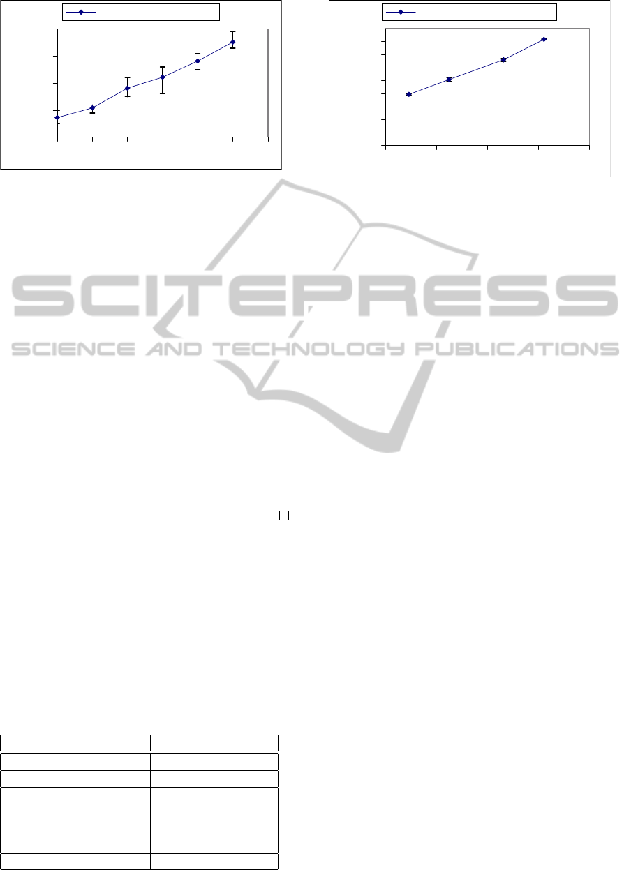
The first test varied the eps value and kept the
same amount of points in each street, i.e., of the orig-
inal dataset that corresponds to 246142 points. The
eps values used were 100, 150, 200, 250, 300 and 350,
while keeping the value of 50 to minPoints. As it was
expected, the Figure 1 shows that with the increase of
eps, the processing time has also increased, because
more points in the neighborhood of a core point could
be expanded.
The Figure 2 illustrates the variation of the num-
ber of points from the input dataset related to the pro-
cessing time. The number of points used was 246142,
324778, 431698 and 510952 points. As expected,
when the number of points processed by DBScan is
increased, the processing time also increases, show-
ing that our solution is scalable.
The Table 2 presents a comparison of our ap-
proach execution time and DBScan centralized ex-
ecution time. We varied the number of points that
was 246142, 324778, 431698 and 510952 points for
eps=100 and minPoints=50. In all cases, our ap-
proach found the same clusters that DBScan central-
ized on the dataset, but spent less time to process as
we expected.
The Figures 3 and 4 show a comparison of our ap-
EfficientandDistributedDBScanAlgorithmUsingMapReducetoDetectDensityAreasonTrafficData
57
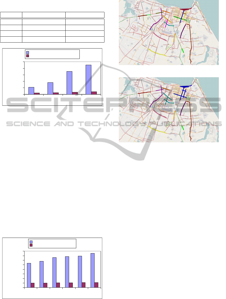
Table 2: Comparing the execution time of our approach and
DBScan centralized for eps=100 and minPoints=50.
Data set Our Approach[ms] Centralized [ms]
246142 197263 1150187.6
324778 254447 2002369
431698 330431 3530966.6
510952 409154 4965999.6
246142 324778 431698 510952
number of points
0
1000000
2000000
3000000
4000000
5000000
processing time (ms)
Data set Variation for DBSCanMR
Data set Variation for Our approach
Figure 3: Varing the dataset size and comparing our ap-
proach with DBSCanMR.
proach and DBScanMR (Dai and Lin, 2012) that has
the partitioning phase centralized, different of our ap-
proach. On the both experiments, our solution spent
less processing time than DBSCanMR, because DB-
SCanMR spends great cost to make the grid during
the centralized partitioning phase.
Moreover, DBSCanMR strategy is sensitive to
two input parameters that are the number of points
that could be processed on memory and a percentage
of points in each partition. For these two parameters,
the paper does not present how they could be calcu-
lated and what are the best values. We did the exper-
iments using the first one equals to 200000 and the
second as 0,49.
We did not compare with the other related work
(He et al., 2011). However, we believe that our ap-
proach presents better results than (He et al., 2011),
because our merge strategy does not need data repli-
cation, that can affect the clustering efficiency for a
100 150 200 250 300 350
eps
0
200000
400000
600000
800000
1000000
1200000
1400000
1600000
processing time (ms)
Eps Variation for DBScanMR
Eps Variation for Our approach
Figure 4: Varing eps and comparing our approach with DB-
SCanMR.
Figure 5: The dataset with 246142 points plotted.
Figure 6: Clusters found after run our approach for 246142
points (eps=100 and minPoints=50).
large dataset.
The Figures 5 presents the points plotted for
246142 points of dataset. Note that each color repre-
sents an avenue of Fortaleza. On the Figure 6, we can
see the clusters found by our approach using eps=100
and minPoints=50. Each cluster found is represented
by a different color on the Figure 6. Note that the
merge occurred where there are more than one avenue
that crosses each other as we expected.
6 CONCLUSION AND FUTURE
WORK
In this paper we proposed a new distributed DBScan
algorithm using MapReduce to identify congested ar-
eas within a city using a large traffic dataset. Our
approach is more efficient than DBSCanMR as con-
firmed by our experiments, while varying the dataset
size and the eps value. We also compare our approach
to a centralized version of DBScan algorithm. Our
approach found the same clusters as the centralized
DBScan algorithm, moreover our approach spent less
time to process, as expected.
As we adopted a distributed processing, the total
time to find the density areas is influenced by machine
ICEIS2014-16thInternationalConferenceonEnterpriseInformationSystems
58

with a worst performance or the one that has more
data to process. So that, our future work will focus on
dealing with data skew because it is fundamental for
achieving adequate data partition. Furthermore, we
will also focus on proposing a partitioning technique
more generic that leads with other kind of data.
REFERENCES
Bentley, J. L. (1975). Multidimensional binary search trees
used for associative searching. In Communications of
the ACM, volume 18, pages 509–517. ACM.
Dai, B.-R. and Lin, I.-C. (2012). Efficient map/reduce-
based dbscan algorithm with optimized data partition.
In Cloud Computing (CLOUD), 2012 IEEE 5th Inter-
national Conference on, pages 59–66. IEEE.
Dean, J. and Ghemawat, S. (2008). Mapreduce: simplified
data processing on large clusters. Communications of
the ACM, 51(1):107–113.
Ester, M., Kriegel, H.-P., Sander, J., and Xu, X. (1996).
A density-based algorithm for discovering clusters in
large spatial databases with noise. In KDD, vol-
ume 96, pages 226–231.
Giannotti, F., Nanni, M., Pedreschi, D., Pinelli, F., Renso,
C., Rinzivillo, S., and Trasarti, R. (2011). Un-
veiling the complexity of human mobility by query-
ing and mining massive trajectory data. The VLDB
JournalThe International Journal on Very Large Data
Bases, 20(5):695–719.
He, Y., Tan, H., Luo, W., Mao, H., Ma, D., Feng, S.,
and Fan, J. (2011). Mr-dbscan: An efficient parallel
density-based clustering algorithm using mapreduce.
In Parallel and Distributed Systems (ICPADS), 2011
IEEE 17th International Conference on, pages 473–
480. IEEE.
Kisilevich, S., Mansmann, F., and Keim, D. (2010). P-
dbscan: a density based clustering algorithm for ex-
ploration and analysis of attractive areas using collec-
tions of geo-tagged photos. In Proceedings of the 1st
International Conference and Exhibition on Comput-
ing for Geospatial Research & Application, page 38.
ACM.
Lin, J. and Dyer, C. (2010). Data-intensive text processing
with mapreduce. Synthesis Lectures on Human Lan-
guage Technologies, 3(1):1–177.
Pavlo, A., Paulson, E., Rasin, A., Abadi, D. J., DeWitt,
D. J., Madden, S., and Stonebraker, M. (2009). A
comparison of approaches to large-scale data analysis.
In Proceedings of the 2009 ACM SIGMOD Interna-
tional Conference on Management of data, SIGMOD
’09, pages 165–178, New York, NY, USA. ACM.
Sousa, F. R. C., Moreira, L. O., Macłdo, J. A. F., and
Machado, J. C. (2010). Gerenciamento de dados em
nuvem: Conceitos, sistemas e desafios. In SBBD,
pages 101–130.
Uncu, O., Gruver, W. A., Kotak, D. B., Sabaz, D., Alib-
hai, Z., and Ng, C. (2006). Gridbscan: Grid density-
based spatial clustering of applications with noise. In
Systems, Man and Cybernetics, 2006. SMC’06. IEEE
International Conference on, volume 4, pages 2976–
2981. IEEE.
White, T. (2012). Hadoop: the definitive guide. O’Reilly.
EfficientandDistributedDBScanAlgorithmUsingMapReducetoDetectDensityAreasonTrafficData
59
