
Approximate String Matching Techniques
Taoxin Peng
1
and Calum Mackay
2
1
School of Computing, Edinburgh Napier University, 10 Colinton Road, Edinburgh, U.K.
2
KANA, Greenock Road, Renfrewshire, U.K.
Keywords: String Matching, Data Quality, Record Matching, Record Linkage, Data Warehousing.
Abstract: Data quality is a key to success for all kinds of businesses that have information applications involved, such
as data integration for data warehouses, text and web mining, information retrieval, search engine for web
applications, etc. In such applications, matching strings is one of the popular tasks. There are a number of
approximate string matching techniques available. However, there is still a problem that remains
unanswered: for a given dataset, how to select an appropriate technique and a threshold value required by
this technique for the purpose of string matching. To challenge this problem, this paper analyses and
evaluates a set of popular token-based string matching techniques on several carefully designed different
datasets. A thorough experimental comparison confirms the statement that there is no clear overall best
technique. However, some techniques do perform significantly better in some cases. Some suggestions have
been presented, which can be used as guidance for researchers and practitioners to select an appropriate
string matching technique and a corresponding threshold value for a given dataset.
1 INTRODUCTION
Data quality is a key to success for all kinds of
businesses that have information applications
involved, such as data integration for data
warehouse applications; text and web mining,
information retrieval and search engines for web
applications. When data need to be integrated from
multiple sources, it always has a problem: how to
identify data records that refer to equivalent entities,
which is called a duplicate detection problem. The
“approximate string matching problem” is generally
used as a black-box function with some threshold
parameter in the context of duplicate detection
problem. In general, string matching deals with the
problem of whether two strings refer to the same
entity.
String matching, also referred as record matching
or record linkage in statistics community has been a
persistent and well-known problem for decades
(Elmagarmid et al., 2007). For a brief review of the
topic of record linkage, see the work by Herzog e
tal., (2010).
To deal with string matching, there are
mainly two types of matching techniques: character-
based and token-based techniques. Character-based
similarity techniques are designed to handle well
typographical errors. However, it is often the case
that typographical conventions lead to
rearrangement of words e.g., “John Smith” vs.
“Smith, John”. In such cases, character-based
techniques fail to capture the similarity of the
entities. Token-based techniques are designed to
compensate for this problem (Elmagarmid et al.,
2007).
Therefore, generally speaking, character-
based similarity techniques are good for the single
word problem, such as name matching while token-
based for the matching with more than one word.
For instance, for e-commerce datasets used in
(Köpcke et al., 2010), token-based techniques could
be more appropriate, given the length of the fields.
This paper will focus on popular token-based
techniques. Although these techniques are designed
for dealing with this kind of problems, since there is
no clear overall best string matching technique for
all kinds of datasets (Christen, 2006), a question still
remains unanswered for researchers and
practitioners: for a given dataset, how to select an
appropriate technique and a threshold value required
by this technique for the purpose of string matching.
In past decade, several researchers have challenged
this problem (Bilenko et al, 2003; Christen, 2006;
Cohen, Ravikumar and Fienberg, 2003;
Hassanzadeh et al., 2007; Peng et al., 2012).
However, none of them have done such a
217
Peng T. and Mackay C..
Approximate String Matching Techniques.
DOI: 10.5220/0004892802170224
In Proceedings of the 16th International Conference on Enterprise Information Systems (ICEIS-2014), pages 217-224
ISBN: 978-989-758-027-7
Copyright
c
2014 SCITEPRESS (Science and Technology Publications, Lda.)

comprehensive analysis and comparison work that is
done for token-based techniques in this paper. The
contributions of this paper are to overview 12
popular token-based string matching techniques,
evaluate whether the following factors will have
effect on the performance: the error rate in a dataset,
the threshold value, the selected type of strings in a
dataset, and the size of a dataset, by using sixty three
carefully designed datasets.
The rest of this paper is structured as follows.
Related works are described in next section. Section
3 introduces techniques that will be examined. The
main contribution of this paper is presented in
section 4 that describes the preparation of the
datasets, the experiments, the analysis and
comparisons. Finally, this paper is concluded and
future work pointed out in section 5.
2 RELATED WORK
Bilenko et al (2003) and Cohen et al., (2003)
evaluated and compared a set of existing string
matching techniques, which include popular
character-based techniques, token-based techniques
and hybrid techniques. They claimed that the
Monge-Elkan performed best on average and
SoftTFIDF performed best overall. However, their
works did not consider the effect of the error rate,
the type of errors in a string, the token length in a
string and the size of a dataset on the performance.
Besides, regarding the threshold value used for
matching, their work only mentioned that a suitable
threshold value was chosen, but not mentioned how
and whether or not this value was universal for all
considered techniques.
Peter Christen (2006) thoroughly discussed the
characteristics of personal names and the potential
sources of variations and errors in them, and also
evaluated a number of commonly used name
matching techniques, considering given names,
surnames and full names separately, and proposed
nine useful recommendations for technique selection
when dealing with name matching problems.
Particularly, the author pointed out the importance
of choosing a suitable threshold value. It was argued
that it was a difficult task to select a proper threshold
value and even small changes of the threshold could
result in dramatic drops in matching quality.
However, his focus was on personal name matching
techniques. Also, similar to Cohen et al’s work
(2003), the author did not consider any effect of the
error rate, the token length in a string and the size of
a dataset on the performance.
Hassanzadeh et al., (2007) presented an overview of
several string matching techniques and thoroughly
evaluated their accuracy on several datasets with
different characteristics and common quality
problems. Similar to this paper, the work was
focused on token-based string matching techniques.
The effect of types of errors and the amount of
errors were both considered. Types of errors
considered include edit errors, token swap and
abbreviation replacement. Their experiment results
showed that types of errors and the amount of errors
both had significant effect on the performance. It
was claimed that the threshold value used for the
matching task would influence the individual
performance of matching techniques. However the
token length in a string and the size of datasets were
not considered.
Recently, Peng et al., (2012) presented an
evaluation work on techniques for name matching.
The work considered a variety of factors, such as the
error rate, the size of a dataset, which might have
effect on the performance of such techniques. Their
preliminary experimental results confirmed that
there is no overall clear best technique. The work
claimed that the error rate in the dataset has effect on
threshold values. However, they only considered
character-based matching techniques.
3 STRING MATCHING
TECHNIQUES
String matching that allows errors is also called
approximate string matching. The problem, in
general, is to “find a text where a text given pattern
occurs, allowing a limited number of “errors” in the
matches.” (Navarro, 2001) Each technique uses a
different error model, which defines how different
two strings are.
In token-based similarities, two strings, s and t
can be converted into two token sets, where each
token is a word. A similarity function, Sim() is used
to define whether strings s and t are similar or not,
based on a given threshold value. In this paper, 12
token-based similarity techniques are considered. In
the rest of this section, if there is no reference given,
the description of algorithm’s formula follows the
work in (Hassanzadeh et al., 2007).
3.1 Notations
Given two relations: R = {r
i
: 1 ≤ i ≤ N
1
} and S = {s
j
: 1 ≤ j ≤ N
2
}, where |R| = N
1
, |S| = N
2
, for a similarity
ICEIS2014-16thInternationalConferenceonEnterpriseInformationSystems
218

function sim( ), a pair of records, (r
i
, s
j
) ∈ R×S is
considered to be similar if sim((r
i
, s
j
) ≥ θ , where θ is
a given threshold value.
3.2 Edit Similarity or Levenshtein
The Levenshtein distance (Navarro, 2001) is defined
to be the minimum number of edit operations
required to transform string s
1
into s
2
. Edit
operations are delete, insert, substitute and copy. It
can be calculated by:
,
1.0
,
max
|
|
,
|
|
where dist(s
1
, s
2
) refers to the actual Levenshtein
distance function which returns a value of 0 if the
strings are the same or a positive number of edits if
they are different. The value of such a measure is
between 0.0 and 1.0 where the bigger the value, the
more similar between the two strings.
3.3 GES
The Gap Edit Similarity (GES) measure uses gap
penalties. (Chaudhuri et al., 2006). GES defines the
similarity between two strings as a minimum cost
required to convert s
1
to s
2
and is given by:
,
1min
,
,1.0
where wt(s
1
) is the sum of weights of all tokens in s
1
and tc(s
1
, s
2
) is a sequence of the following
transformation operations:
Token insertion: inserting a token t in s
1
with
cost w(t). c
ins
where c
ins
is the insertion factor
constant and is in the range between 0 and 1. In
our experiments, c
ins
=1;
Token deletion: deleting a token t from s
1
with
cost w(t);
Token replacement: replacing a token t
1
by t
2
in
s
1
with cost (1- sim
Leven
(t
1
, t
2
).w(t).
3.4 Jaccard/Weighted Jaccard
Jaccard similarity is the fraction of tokens in s
1
and
s
2
that are present in both of the strings. Weighted
Jaccard similariy is the weighted version of Jaccard
similarity. The similarity measure for two strings, s
1
,
s
2
can be calculated by:
.
,
∑
∈
∩
∑
∈
∪
where w
R
(t) is a function of weight that reflects the
frequency of token t in relation R:
log
0.5
0.5
where n is the number of tuples in the relation R and
n
t
is the number of tuples in R containing the token t.
3.5 TF-IDF
TF-IDF, term frequency–inverse document
frequency, is a similarity measure that is widely used
in information retrieval community (Cohen,
Ravikumar and Fienberg, 2003). The similarity
measure for two strings, s
1
, s
2
can be calculated by:
,
,
∙,
∈
∩
together with:
,
log
,
1∙log
and
,
,/
,
where TF
w, s
is the frequency of token w in s, IDF
w
is
the inverse of the fraction of names in the corpus
that contains w.
3.6 SoftTFIDF
SoftTFIDF is a hybrid similarity measure by Cohen
et al., (2003), in which similar tokens are considered
as well as tokens in s
1
s
2
. The similarity measure
for two strings, s
1
, s
2
can be calculated by:
,
,
∙,
∙,
∈,
,
where CLOSE(θ, s
1
, s
2
) is the set of tokens t
1
∈s
1
such that for some t
2
s
2
sim(s
1
, s
2
)>θ, where sim() is
a secondary similarity function, and D(w, s
2
) =
max
v
∈
s2
sim(w, s
2
), for w∈CLOSE(θ, s
1
, s
2
).In the
experiments, Jaro-Winkler similarity function is
used as the secondary similarity function and θ =
0.9.
3.7 Cosine TF-IDF
Cosine TF-IDF is a well-established technique used
in Information Retrieval and uses vectors to analyse
the strings and to calculate the similarity between
the pattern and the string. The similarity is
determined by the cosine of the angle between these
vectors. The formula is shown below for the
ApproximateStringMatchingTechniques
219

similarity, as well as the formula for how the vectors
are assigned:
,
∙
∈
∩
where
(t) and
are normalized tf-idf
weights for each common token in s
1
and s
2
respectively. The normalized tf-idf weight of token
t in a given string s is defined as follows:
∑
∈
,
∙
where
is the term frequency of token t within
string s and idf(t) is the inverse document frequency
with respect to the entire relation R.
3.8 BM25
BM25 is an efficient string searching technique that
is used as the foundation for many others. The
algorithm looks for instances of P (pattern) in S
(text) by performing comparisons of characters at a
range of different alignments. The similarity
measure for two strings, s
1
, s
2
can be calculated by:
,
∙
∈
∩
where
1∙
1∙
and
log
0.5
0.5
1
|
|
where tf
s
(t) is the frequency of the token t in string s,
|s| is the number of tokens in s, avg
s
is the average
number of tokens per record in relation R, n
t
is the
number of records containing the token t and k
1
, k
2
and b are a set of indpendent parameters, where k
1
∈
[1,2], k
2
= 8 and b∈ [0.6, 0.75].
3.9 Hidden Markov
Hidden Markov Model (HMM) has a formula
wherein a language model is given to each
individual document. HMM is a model that is
assigned to actual strings whereby the probability of
returning a particular string is measured against
another string. The following formula shows the
score for HMM used in this experiment:
,
|
|
∈
where a
0
and a
1
= 1 - a
0
are the transition states
probabilities of the Markov model and P(t|GE) and
P(t|s
2
) are determined by:
|
∑
∈
∑
||
∈
|
|
|
3.10 WHIRL
The similarity of two document vectors
v
and
w
is
usually interpreted as the cosine of the angle
between v and w. The value of Sim
WHIRL
(
v
,
w
) is
always between one and zero and is given by the
following formula (Cohen, 2000):
,
∙
|
|
|
|∙|
|
|
|
∈
where
v
is related to the “importance” of the term t
in the document represented by
t
and is related
to the relevance of term t in the document
represented by
t.
is the length of vector
and is the length of the vector Two
documents are similar when they share many
“important” terms (Cohen, 2000).
3.11 Affine Gap
Some sequences are much more likely to have a big
gap, rather than many small gaps. For example, a
biological sequence is much more likely to have one
big gap of length 10, due to a single insertion or
deletion event, than it is to have 10 small gaps of
length 1. Affine gap penalties use a gap opening
penalty, o, and a gap extension penalty, e. A gap of
length l is then given a penalty o + (l-1)e. So that
gaps are discouraged, o is almost always negative.
Because a few large gaps are better than many small
gaps, e, though negative, is almost always less
negative than o, so as to encourage gap extension,
rather than gap introduction.
In the Affine Gap Penalty model, a gap is given a
weight Wg to “open gap” and another weight Ws to
“extend the gap”. The formula for the model is:
v
w
w
|||| v
v
|||| w
.w
ICEIS2014-16thInternationalConferenceonEnterpriseInformationSystems
220

where q is the length of the gap, W
g
is the weight to
“open the gap” and W
s
is the weight to “extend the
gap” with one more space (Vingron and Waterman,
1994).
3.12 Fellegi-Sunter
Fellegi-Sunter makes comparison between recorded
characteristics and values in two records and makes
a decision based on whether or not the comparison
pair make up the same object or event (Fellegi and
Sunter, 1969).
Decisions are made according to three types
which will be referred to as A
1
(a link)
,
A
2
(a possible
link) and A3(a non-link). When members of the
comparison pair are unmatched then Fellegi-sunter
equation calculates the score by determining the
probability of the error occurring between the
matched pair defined as:
|
∈
|
∈
where u(γ) and m(γ) are probabilities of realizing
and discovering a comparison vector. The
summation is the total space P of all possible
realizations.
4 EXPERIMENTS AND
EVALUATION
In our experiments, we focus on the performance of
the above 12 popular token-based string matching
techniques. Datasets designed cover a wide range of
characteristics, such as the level of “dirtiness”, the
token length in a string, the size of datasets and the
type of errors. It is expected that the experiment
results should show that all these characteristics
have significant effect on the performance and
optimal threshold values.
4.1 Datasets Preparation
In the absence of common datasets for data cleaning,
we prepare our data for experiments as follows.
The datasets that are used are based on real
Electoral Roll data. First, a one million record
dataset was extracted, from which an address list
was created, which includes House number, Street,
City and County, Postcode. This list contains 10000
clean, non-duplicate addresses, with an ID
associated to each of the records.
Erroneous records were introduced by doing the
following five operations manually to the address
fields of records: inserting, deleting, substituting,
replacing characters and swapping tokens. The
replacing type of errors includes abbreviation errors,
such as replacing St. with Street or vice versa. The
level of the dirtiness of a dataset is divided into three
levels: Low, Medium and High. Static percentages
are used as a guideline for such a classification: for
low error datasets, the percentage was set to 20%;
for medium, 50% and for high, 80%.
The dataset sizes that were considered consisted
of six sizes with 500, 1000, 2000, 4000, 8000 and
10000 records respectively. The average record
length was approximately 8.2 words per record. The
errors in the datasets were distributed in a uniform
way. Experiments have also been run on datasets
generated using different parameters. For each size,
there were three datasets generated with mixed types
of errors, having a different error rate associated.
This contributes eighteen datasets with mixed type
of errors introduced.
In addition, datasets with single type of errors
were also considered in our experiment. The
insertion and deletion errors were incorporated
solely into each dataset and the algorithms were
measured against each other to see how they
performed against each technique. With regard to
how these error types were distributed amongst the
data, the distribution went as follows: Insertion
errors were performed on a single character per
record that would correspond to a given percentage
distribution rate dependent on the error rate being
analyzed. For example, for the low error dataset for
1000 records, there were 20% of those records that
had a single “insertion” error implemented. So 200
of those 1000 records had a character “added” that
would simulate an error. There were 18 datasets
incorporated with only insertion errors.
Deletion followed a similar approach for each
error rate and took a single character away from the
number of records corresponding to the respective
percentage error rate. There were 18 such datasets as
well.
Token lengths were measured for the 8000 size
dataset with the “low”, “medium” and “high” error
rates taken into consideration. Three different token
lengths were used, “Short”, “Medium” and “Long”.
For the short tokens, the only fields considered for
each record were for Street and City. Medium length
considered County and the Long length size added
PostCode which was the original size of the record.
ApproximateStringMatchingTechniques
221
The average length used for low was 2.1 tokens per
record, medium was 5.6 and long was 8.2. Therefore
in total there are sixty three datasets for the
experiment.
4.2 Measures
A target string is a positive if it is returned by a
technique; otherwise it is a negative. A positive is a
true positive if the match does in fact denote the
same entity; otherwise it is a false positive. A
negative is a false negative if the un-match does in
fact denote the same entity; otherwise it is a true
negative.
We evaluate the matching quality using the F-
measure (F) that is based on precision and recall:
1
2
with P (precision) and R (recall) defined as:
||
|
|
|
|
||
|
|
|
|
Clearly, a trade-off between recall and precision
exists, if most targets are matched, recall will be
high but precision will be low. Conversely if
precision is high, recall will be low. F1-measure is a
way of combining the recall and precision into a
single measure of overall performance (Rijsbergen,
1979). In our experiments, precision, recall and F1-
measure are measured against different value of
similarity thresholds, θ. For the comparison of
different techniques, the maximum F1-measure
score across different thresholds is used.
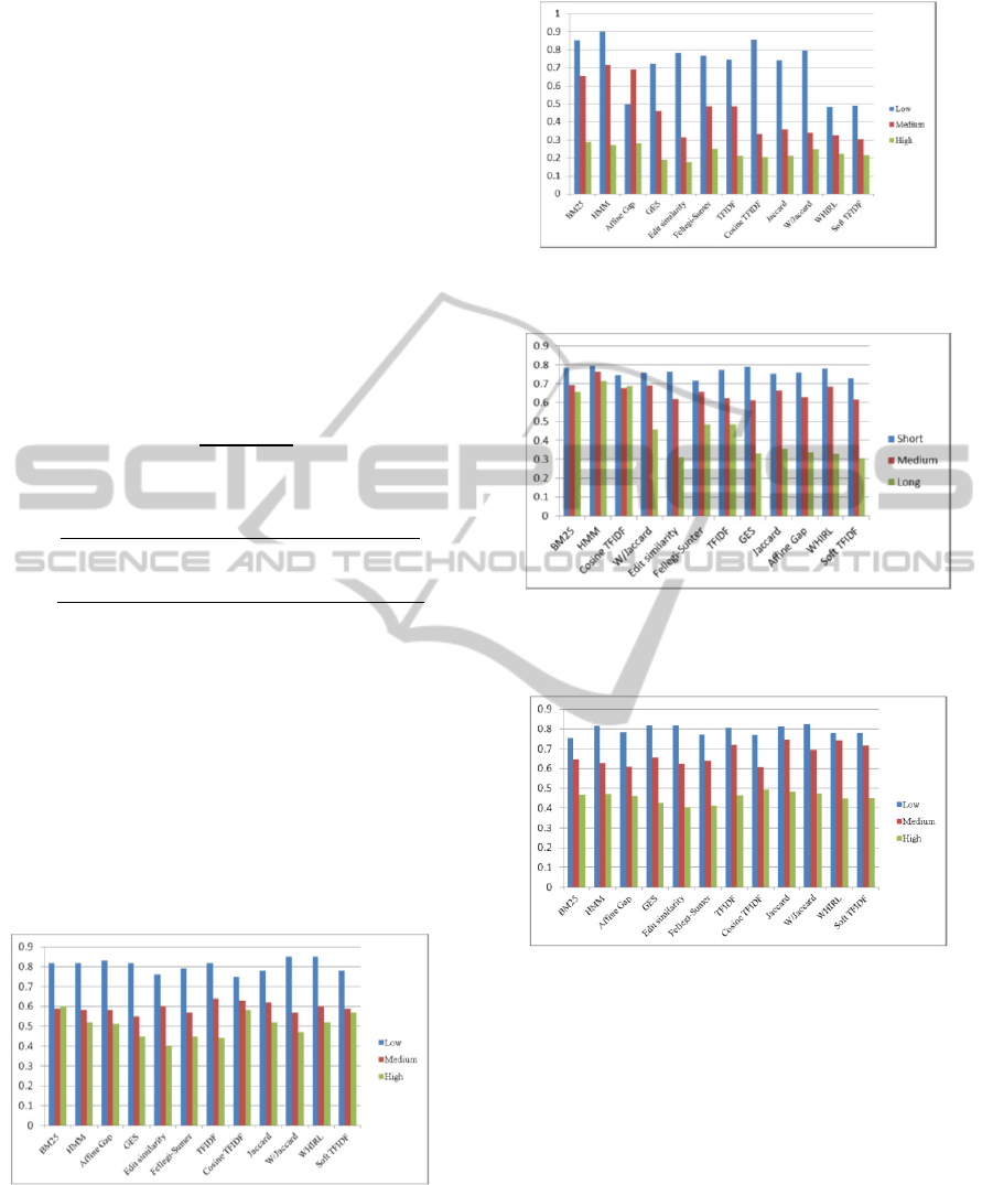
Figure 1: Optimum threshold value for different
techniques on datasets with three different error rates.
Figure 2: Maximum F1- score for different techniques on
datasets of 8000 records with three different error rates.
Figure 3: Maximum F1- score for different techniques on
datasets of 8000 records with three different token length
associated with medium error rates.
Figure 4: Maximum F1- score for different techniques on
datasets of 10000 records only having insertion errors with
three different error rates.
4.3 Results
In this section, testing results on the sixty three
carefully designed datasets are analysed and
evaluated. Results show that in general, the size of a
dataset is not significantly sensitive to the accuracy
(the best F1-score) relative to the threshold values.
4.3.1 Effect of Error Rate on Threshold
Values
Figure 1 shows the optimum threshold values for all
12 techniques on datasets with three different error
ICEIS2014-16thInternationalConferenceonEnterpriseInformationSystems
222

rates. The results confirm that the level of “dirtiness”
in a dataset has significant effect on threshold
selection. From the figure, it says the higher the
error rate in the dataset, the lower the threshold
value is required in order to achieve the maximum
F1-score, except the case for BM25. For example
W/Jaccard achieves the maximum F1-score on
datasets with low error rate at the threshold value of
0.85, with medium and high error rate at threshold
values of 0.57 and 0.47 respectively. However,
BM25 achieves the maximum F1-score on datasets
with high error rate at the threshold value of 0.60,
but with medium error rate at the threshold value of
0.59.
4.3.2 Effect of Error Rate on Performance
Experiment results show that the “dirtiness” of a
dataset has great effect on the overall performance.
As an example, Figure 2 shows the maximum F1-
scores for the 12 different techniques on datasets of
size 8000 with three different error rate associated. It
shows that for datasets with low error rate
associated, HMM, BM25 and Cosine TF-IDF are the
best three performers among the 12 algorithms,
while Affine Gap, WHIRL and SoftTFIDF are the
worst performers. For datasets with medium and
high error rate associated, Affine Gap joined HMM
and BM25 as the top three performers, while Cosine
TF-IDF drops out of the best 5. This shows that
Affine Gap is suitable for datasets with higher level
of “dirtiness”, and Cosine TF-IDF is suitable for
datasets with lower level of “dirtiness”. In general,
the performance decreases along with the increase of
the “dirtiness” in a dataset, except technique, Affine
Gap, which has higher maximum F1-score on
datasets with medium error rate associated than on
datasets with low error rate associated.
4.3.3 Effect of Size of Datasets on
Performance
Our experiment results show that the size of datasets
does not have significant effect on maximum F1-
score values, given optimum threshold values.
4.3.4 Effect of Length of Strings on
Threshold Values
Figure 3 shows the maximum F1- score for different
techniques on datasets of 8000 records with three
different token lengths associated with medium error
rates. It says in general, performance decreases
along with the increase of lengths, except Cosine
TF-IDF, where the performance on long length
datasets is slightly better than that on medium
length. From results for different techniques on
datasets with medium length and long length tokens
respectively, associated with three different error
rate, it can be seen that BM25, HMM, cosine TF-
IDF and W/Jaccard performed better than others,
and Affine Gap, WHIRL and SoftTFIDF performed
badly when the token length is long, However, the
performance of Affine Gap, WHIRL and SoftTFIDF
increased significantly when the token length is
medium.
4.3.5 Effect of Type of Errors on
Performance
Figure 4 shows the maximum F- score for different
techniques on datasets of 10000 records only having
insertion errors with three different error rates. For
datasets with low error rate associated, W/Jaccard,
GES and Edit Similarity are the best three
performers, while Fellegi-Sunter, Cosine TF-IDF
and BM25 perform worse than the rest. The
performance of BM25 increases along with the
increase of the level of “dirtiness” in datasets, while
the performance of GES and Edit Similarity
decreases along with the increase of the level of
“dirtiness” in datasets. It is noted that BM25 is
among the best three performers in most of cases
when the error types in datasets are mixed. See
section 4.3.2.
4.3.6 Effect of Timing
Results also show, when the error rate is low,
Affine, GES, Felligi-Sunter and Edit Similarity cost
less time among the twelve algorithms whereas
SoftTFIDF costs the most time. The pattern is
similar when the error rate is medium. However,
SoftTFIDF costs the least time when the error rate is
high. HMM, TF-IDF and WHIRL also cost less time
than the rest when the error rate is high. Our
experiment results agree that smaller datasets cost
less time, and the time used increases when the error
rate increases. In particular, time used on datasets
with high error rate associated is significantly more
than that on datasets with low or medium error rate
associated.
4 CONCLUSIONS AND FUTURE
WORK
This paper has analysed and evaluated twelve
popular token-based name string matching
ApproximateStringMatchingTechniques
223

techniques. A comprehensive comparison of the
twelve techniques has been done based on a series of
experiments on 63 carefully designed datasets with
different characteristics, such as the rate of errors, the
type of error, the number, the length of tokens in a
string, and the size of a dataset. The comparison
results confirmed the statement that there is no clear
best technique. The characteristics considered all
have significant effect on performance of these
techniques, except the size of a dataset. In general,
HMM and BM25 perform better than others,
especially on smaller sized datasets, but consume
much more time. Cosine TF-IDF and TF-IDF are
better on larger datasets with a higher error rate
associated. Results also show that techniques that
perform well on datasets incorporated with mixed
type of errors do not secure a similar performance on
datasets incorporated with a single type of errors. For
example, BM25 didn’t perform well on datasets with
low error rate, incorporated only with insertion
errors. Similarly, HMM didn’t perform well on
datasets with low error rate, incorporated with only
deletion errors. The token length also has an effect on
the performance. For example, some techniques,
such as Affine Gap, WHIRL and SoftTFIDF
performed much better when the token length is
medium than that of the token length when it is long.
Regarding the threshold value, the results show
that the level of “dirtiness” in a dataset has
significant effect on threshold selection. In general,
the higher the error rate in the dataset, the lower the
threshold value is required in order to achieve the
maximum F1-score.
The work introduces a number of further
investigations, including: 1) to do more experiments
on datasets with more characteristics, such as the
number of tokens in strings etc.; 2) to do further
analysis in order to evaluate whether there is a
method to select a threshold value for any of the
matching techniques on a given dataset.
REFERENCES
Bilenko, M., Mooney, R., Cohen, W., Ravikumar, P. and
Fienberg, S., 2003. Adaptive Name Matching in
Information Integration, IEEE Intelligent Systems, vol.
18, no. 5, pp. 16-23.
Chaudhuri, S., Ganti, V. and Kaushik, R., 2006. A
primitive operator for similarity joins in data cleaning.
In Proceedings of International Conference on Data
Engineering.
Christen, P., 2006. A Comparison of Personal Name
Matching: Techniques and Practical Issues. In
Proceedings of the Sixth IEEE International
Conference on Data Mining - Workshops (ICDMW
'06). IEEE Computer Society, Washington, DC, USA,
pp.290-294.
Cohen, W., 2000. WHIRL: A word-based information
representation language. Artificial Intelligence,
Volume 118, Issues 1-2, pp. 163-196.
Cohen, W., Ravikumar, P. and S. Fienberg., 2003. A
comparison of string distance metrics for name-
matching tasks. In Proceedings of the IJCAI-2003
Workshop on Information Integration on the Web,
pp.73-78.
Elmagarmid, A., Ipeirotis, P. and Verykios, V., 2007.
Duplicate Record Detection: A Survey. IEEE Trans.
Knowl.Data Eng., Vol.19, No.1, pp. 1-16.
Fellegi, P. and Sunter, B., 1969. A Theory for Record
Linkage. Journal of the American Statistical
Association, 64(328), pp. 1183-1210.
Hassanzadeh, O., Sadoghi, M. and Miller, R., 2007.
Accuracy of Approximate String Joins Using Grams.
In Proceedings of QDB'2007, pp. 11-18.
Herzog, T., Scheuren, F. and Winkler, W., 2010, “Record
Linkage,” in (D. W. Scott, Y. Said, and E.Wegman,
eds.)Wiley Interdisciplinary Reviews: Computational
Statistics, New York, N. Y.: Wiley, 2 (5),
September/October, 535-543.
Köpcke, H., Thor, A., and Rahm, E., 2010. Evaluation of
Entity Resolution Approahces on Real-world Match
Problems, In Proceedings of the VLDB Endowment,
Vol. 3, No. 1.
Navarro, G., 2001. A Guide Tour to Approximate String
Matching. ACM Computing Surveys, Vol. 33, No. 1,
pp. 31–88.
Peng,T., Li, L. and Kennedy, J., 2012. A Comparison of
Techniques for Name Matching. GSTF International
Journal on Computing , Vol.2 No. 1, pp. 55 - 61.
Rijsbergen, C., 1979. Information Retrieval. 2
nd
ed.,
London: Butterworths.
Vingron, M. and Waterman, S., 1994. Sequence alignment
and penalty choice. Review of concepts, case studies
and implications. Journal of molecular biology 235
(1), pp. 1–12.
ICEIS2014-16thInternationalConferenceonEnterpriseInformationSystems
224
