Neural Network for Fretting Wear Modeling

Laura Haviez

1,2,3

, Rosario Toscano

, Siegfried Fourvy

and Ghislain Yantio

LTDS, UMR 5513, Ecole Centrale de Lyon, Ecully, France

LTDS, UMR 5513, ENISE, Saint-Etienne, France

SAGEM, Boulogne-Billancourt Cedex, France

Keywords: Fretting Wear Modeling, Artificial Intelligence, Artificial Neural Networks.

Abstract: Materials wear is a very complex, only partially-formalized phenomenon involving numerous parameters

and damage mechanisms. The need to characterize wear in many industrial applications prompted the

present research. The study concerns an original strategy investigating the effect of contact conditions on

the wear behavior of carburized stainless steels under fretting and reciprocating sliding motion. A physical

model was constructed, and pre-treated experimental data were incorporated in a neural network to model

wear volume. Three models are proposed and compared, according to input.

1 INTRODUCTION

Wear is generally defined as loss of surface material

from contact surfaces subjected to relative motion.

Tribologic issue must therefore be taken into

consideration, and several models have been

developed in recent years (Kolodziejczyk, 2010;

Zhang, 2003). These models usually correlate wear

volume with physical and geometrical quantities

such as load, sliding distance, coefficient of friction,

hardness, materials (Anand Kumar, 2013; Genel,

2003; Sahraoui, 2004), and physical laws such as the

Archard wear criterion (Archard, 1953). Many

parameters influence wear. To identify one relevant

parameter, we chose a neural network to model

wear, creating an experimental database: the great

advantage of Artificial Neural Networks (ANNs) is

their ability to be used as an arbitrary function

approximation mechanism which ‘learns’ from

observed data. Fretting damage was used as a case

study. Small oscillatory movements may induce

interface fretting, shortening predicted lifetime. The

interface wear response was modeled and empirical

models were created based on data from fretting

tests. The Artificial Intelligence model was validated

against the physical description of fretting wear

behavior.

2 EXPERIMENTAL PROCEDURE

2.1 Material and Contact Type

Tests were performed on two chromium-

molybdenum stainless steels: one carburized

stainless steel (M1) and one stainless steel with mass

quenching (M2). The M1 specimen comprised 3

layers: the external layer was hard and decarburized

layer (white layer: WL); the second was the

carburized phase (CL), with hardness gradient

between 760 HV and 550HV (Figure 1a); the third

was the bulk, with 500 HV hardness. These

materials were studied to determine the wear

kinetics of a two cross-cylinder configuration.

According to Hertz, this configuration is equivalent

to a sphere/plane configuration where M1 is mobile

and M2 fixed. The two cylinders had the same

radius (7.5 mm) and the same length (20 mm). The

normal force was adjusted to reach 2,200 MPa

Hertzian maximum contact pressure. Surface

roughness was Ra=0.4µm for both materials.

2.2 Test System

Figure 1b shows a diagram of the fretting wear test.

An MTS hydraulic tension-compression machine

regulated displacement between cylinders (further

details of this setup and experimental method used

can be found in (Fouvry, 1996)). During the test,

normal force P was kept constant by a feedback

617

Haviez L., Toscano R., Fourvy S. and Yantio G..

Neural Network for Fretting Wear Modeling.

DOI: 10.5220/0004908506170621

In Proceedings of the 6th International Conference on Agents and Artiﬁcial Intelligence (ICAART-2014), pages 617-621

ISBN: 978-989-758-015-4

 2014 SCITEPRESS (Science and Technology Publications, Lda.)

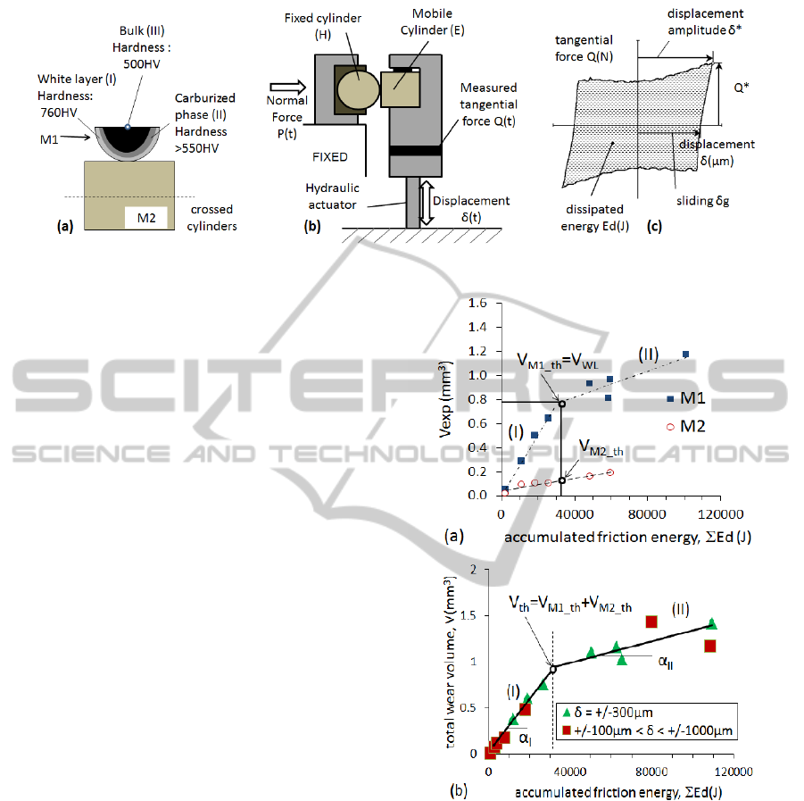
Figure 1: (a) Contact configuration (crossed cylinders); (b) Fretting setup; (c) Fretting cycle analysis.

system, and the cyclic sinusoidal displacement δ*

was applied to generate an alternating tangential

load Q* on the contact. All tests were performed

with a constant frequency of 3 Hz, at room

temperature. This enabled the fretting loop Q-δ to be

plotted for chosen cycles (Figure 1c). During tests,

displacement amplitude was fixed between ±100µm

and ±1000µm, leading to two generalized slip

regimes: gross slip in fretting, and reciprocating. The

first tests were performed with ±300µm

displacement and different numbers of cycles, and

the second with different displacement amplitudes

δ* and numbers of cycles N. Because of system

stiffness, the sliding amplitude δg was not always

the same for a given displacement amplitude. For

each test, slip was generalized in the interface, and

the ratio Q*/P was supposed to be constant for any

displacement amplitude.

The ratio Q*/P was then defined as the

coefficient of friction µ, and the dissipated energy

Ed during the fretting cycle was given by the area of

the corresponding hysteresis cycle (see Figure 1c).

The accumulated friction energy was determined by

summing friction loop energy over the whole test

duration:





4...μ.



(1)

Wear volume (V) after testing was measured on a

3D scan. Wear rate was established from wear

volume versus accumulated friction energy

(Archard, 1953). Figure 2a compares evolution of

wear volume in M1 and M2 specimens versus

accumulated friction energy. Wear volume evolution

was linear in M2 but showed a bilinear tendency in

M1, linked to the structure of the M1 interface

(Figure 1a): wears initially involved the brittle white

layer of M1 (WL) before reaching the subsurface

carburized layer (CL), the wear rate was lower. It is

noteworthy that, while the wear rate in the counter-

Figure 2: (a) Evolution of wear volume VM1 and VM2;

(b) Total wear volume evolution (V=VM1 + VM2) versus

accumulated friction energy (Vth; αI and αII are defined

from the δ=±300µm experiments).

body was equivalent to that of the M1

layer (II),

that of the M1 top WL layer (I) displayed

significantly (approx. 10-fold) higher wear kinetics.

Total wear volume V = V

+ V

is related to

total accumulated friction energy (Figure 2b).

Considering the difference between the top WL

response and sub-carburized layer, a bilinear energy

wear model can be introduced as follows:

 If V < V

, the interface involves the M1

domain, and V

= α

. ΣEd

ICAART2014-InternationalConferenceonAgentsandArtificialIntelligence

618

 If V > V

, all the M1

phase has been

worn out and the interface involves only the

sub-carburized layer, and V

= α

(ΣEd-Ed

) + V

where Ed

/ α

, V

is the threshold wear volume

related to M1 white layer elimination (V

) plus

associated M2 wear. V

can be expressed as a

function of the contact area A

and the white layer

thickness (h

) (i.e., V

. Af), where α

is the

energy wear rate of the M2/M1

interface, and α

is the energy wear rate of the M2/M1

interface.

Using this very simple physical model involving

only 3 material parameters (V

, α

and

), it is

possible to express the total wear kinetics of the

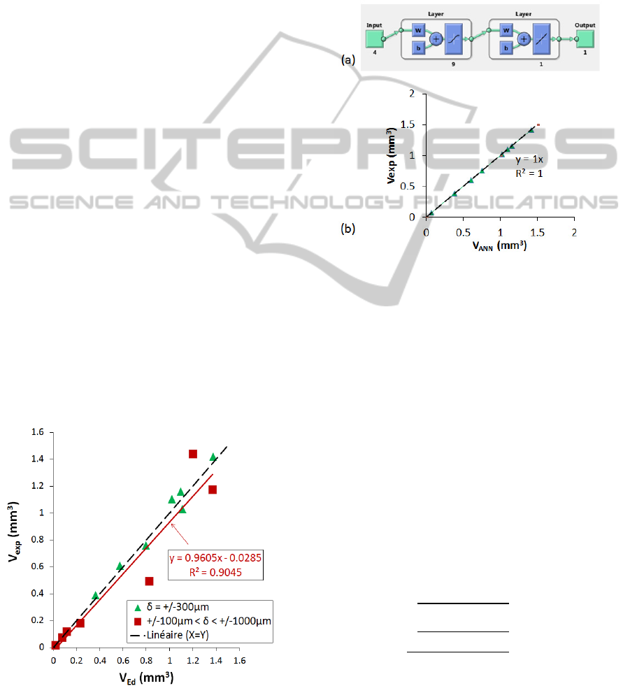
interface. The theoretical description is compared

with the experimental results in Figure 3. The results

related to δ*=+/-300µm fretting sliding are also

compared with other results for fretting and large

reciprocating sliding conditions. The regression

coefficient is about R²=0.9045, which confirms the

stability of the energy approach to formalizing wear

rate even for a complex interface like that

investigated here.

3 MODELING WEAR

EVOLUTION

This wear behavior could not be predicted or

expected initially, because of the bi-linear

phenomenon, for which a static Neural Network was

used to estimate wear evolution as a function of

dissipated energy Ed with respect to mechanical

variables and environmental conditions (Figure 4). A

Figure 3: Comparison of experimental (Vexp) and

theoretical (VEd) wear volume.

dynamic Neural Network could not be used because

of the poor database. We propose 3 models with

different key input parameters. The input data are P,

δg, µ and N for the first network (Model_A), only

Ed for the second (Model_B) and a combination of

all 5 parameters for the third (Model_C). Model_A

and Model_B could be expected to give the same

results, as Ed can be approximated by the inputs of

Model_A as shown in Eq.1.

Figure 4: (a) Schematic description of the network

structure; (b) Network training results.

The structure adopted was a two layer network with

9 neurons in the hidden layer and 1 in the output

layer (Figure 4a). For the input layer, the transfer

function was a sigmoidal tangent (tansig), and for

the last layer a linear function (purelin).

The three models were assessed by comparing

experimental and predicted wear volume. The

experiments performed with ±300µm displacement

amplitude with different numbers of cycles

constituted training data, and the other experiments

(±100µm to ±1,000µm with different numbers of

cycles) represent the test data. Simulation could be

expected to be difficult, as the network could not be

trained on the variable δg. Figure 4b, however,

shows excellent network training, with R²=1 for

each model. To compare the models, the percentage

square root of normalized variance was defined as

follows:







∑

















∗

(2)

where Xi is the experimental wear data, Ui the

predicted wear data, Z the number of samples, and

max

the maximum experimental wear volume.

NeuralNetworkforFrettingWearModeling

619

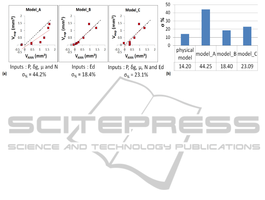
Figure 5: (a) Test results of the three Neural Networks; (b) Variance results of the physical model and the three ANN

models.

4 RESULTS AND DISCUSSION

The variance σ of the physical energy wear model

was about 14.2 % (Figure 3). All simulated wear

volume results for the 3 models are presented in

Figure 5a.

Model_A was unable to predict wear volume, as

the correlation was poor (σ = 44.2%). Model_B had

only Ed input, the key parameter in this study;

correlation was excellent (σ = 18.4%) and only 4.2%

different from the experimental correlation. The

input variables used in Model_A could be used to

calculate the dissipated energy Ed (Eq.1), whereas

the neural network could not achieve this internally

to give a good estimate of wear volume, probably

due to the small amount of data available for

network training. Model_B was more reliable than

Model_A. In Model_C, all the parameters are

considered as inputs; the linear regression R² was

better than in the other models, but the dispersion

was greater (σ = 23.1%); wear prediction for low

accumulated dissipated energy was poorer than in

Model_A, but for higher energy the results were

similar to those of Model_B.

5 CONCLUSIONS

A static Artificial Neural Network was built and

validated for variable fretting and reciprocating

conditions. In-situ wear volume measurement

enabled a model describing wear behavior to be

created, providing reliable simulation of wear. The

ANN model assessed wear volume almost as well as

the physical model (Figure 5b) in spite of the small

amount of experimental data. At this point in the

study, it is difficult to choose between Model_B and

Model_C: one had a better correlation factor,

whereas the other had less dispersion. Model_B

provided better wear prediction for low accumulated

dissipated energy. However, this issue needs more

investigation. Another crucial issue is the size of the

database used for the training and the test; this is a

recurrent problem in many industrial applications,

where the amount of data is insufficient for effective

parameterization of standard neural structures. In

such situations, one possible approach is to consider

the hidden layer as “simply” a projection operator,

given which learning could be performed on the

output layer alone. These aspects (projection

operator and output learning) need to be investigated

more precisely to optimize estimation of wear

volume.

REFERENCES

Anand Kumar S., Ganesh Sundara Raman S., Sankara

Narayanan T. S. N., Gnanamoorthy R., 2013.

Materials and Design. Prediction of fretting wear

behavior of surface mechanical attrition treated Ti–

6Al–4V using artificial neural network. Volume 49,

Pages 992–999.

Archard J. F., 1953, Journal of Applied Physics. Contact

and Rubbing of Flat Surfaces. Volume 24(8), Pages

981-988.

Fouvry S., Kapsa Ph., Vincent L., 1996. Wear.

Quantification of fretting damage. Volume 200, Pages

186-205.

Genel K., Kurnaz S. C., Durman M., 2003, Materials

Science and Engineering. Modeling of tribological

properties of alumina fiber reinforced zinc–aluminum

composites using artificial neural network. Volume

A363, Pages 203–210.

Kolodziejczyk T., Toscano R., Fouvry S., Morales-Espejel

G., 2010. Wear. Artificial intelligence as efficient

ICAART2014-InternationalConferenceonAgentsandArtificialIntelligence

620

technique for ball bearing fretting wear damage

prediction. Volume 268, Issues 1–2, Pages 309-315.

Sahraoui T., Guessasma S., Fenineche N.E., Montavon G.,

Coddet C., 2004. Materials Letters. Friction and wear

behaviour prediction of HVOF coatings and

electroplated hard chromium using neural

computation. Volume 48, Pages 654– 660.

Zhang Z., Barkoula N.-M., Karger-Kocsis J., Friedrich K.,

2003. Wear. Artificial neural network predictions on

erosive wear of polymers. Volume 255, Pages708–

713.

NeuralNetworkforFrettingWearModeling

621