
First Heart Sound Detection Methods
A Comparison of Wavelet Transform and Fourier Analysis in Different
Frequency Bands
P. Langer
1,2
, P. Jurák
2
, J. Halámek
2
and V. Vondra
2
1
International Clinical Research Center, Brno, Czech Republic
2
Institute of Scientific Instruments AS CR, Brno, Czech Republic
Keywords: First Heart Sound, Respiration, Stroke Volume, Correlation, Wavelet Transform, Fourier Analysis.
Abstract: Methods of heart sound pre-processing are compared in this study. These methods are wavelet transform
and Fourier analysis in different frequency bands. After pre-processing, the first heart sound was detected.
Correlation of the first heart sound with respiration was chosen, as a sign of optimal detection. The results
are demonstrated in a study of 30 volunteers. Optimal band selection for heart sound filtering is shown to be
strongly individual, and is far more important than selecting Fourier analysis or wavelet transform as
filtering method. Correlation with respiration proved to be a good sign for first heart sound detection
evaluation.
1 INTRODUCTION
Evaluation of heart sound has been used for
diagnosis for a long time. Despite advances in ECG
it still has the potential to provide a cost-effective
technology for monitoring valuable information
about the heart. Normally, the heart sound is made
up of two separated sounds, the first and the second
heart sound. Together, they are known as the
fundamental heart sound (FHS). According to
valvular theory FHS emanate from a source located
near the valves. However, cardiohaemic theory says
that the heart and blood are an interdependent
system that vibrates as a whole (Smith and Craige
1988). When we focus on valvular theory, the first
heart sound (S1) is caused by closure of the
atrioventricular valves at the beginning of
ventricular contraction, thus identifying early
systole. The second heart sound (S2) is caused by
closure of the semilunar valves at the end of
ventricular systole. The time between S1 and S2 is
known as left ventricular ejection time (LVET) or
systole. LVET is an important parameter in number
of applications such as computing left ventricular
stroke volume (SV) according to (Bernstein and
Lemmens, 2005; Cybulski, 2011). One possible way
of computing SV is represented by equation (1). In
addition to LVET, the maximum of derived thorax
impedance
⁄
, raw thorax impedance
, and a constant based on body weight, height and
thorax volume
ζ
⁄
are also used for SV
calculation. When we realize that the changes in
value are minimal, there are just two parameters that
influence SV, namely
⁄
and LVET.
Accurate detection of S1 and S2 is therefore crucial
for correct definition of LVET and SV.
ζ
2
⁄
(1)
Heart sound is a highly non-stationary and complex
signal. S1 consists of two main components, the
closure of the mitral valve (M1) and the closure of
the tricuspid valve (T1) (Debbal and Bereksi-Reguig
2008), as shown in Figure 1. S1 has quite a stable
position within the R-R interval. It is located from
the R-wave + 5 % of the R-R distance to the R-wave
+ 20 % of the R-R distance, abbreviated to 0.05R-R
to 0.2R-R (El-Segaier et al 2005). Information
concerning the spectrum of the S1 is not clear in the
literature. One source claims the spectrum is in the
interval 50–150 Hz (Abdelghani and Fethi 2000),
another source claims 20–150 Hz (JiZhong and
Scalzo 2013).
Many studies have tried to find a successful
automated heart sound classification algorithm. The
278
Langer P., Jurák P., Halámek J. and Vondra V..
First Heart Sound Detection Methods - A Comparison of Wavelet Transform and Fourier Analysis in Different Frequency Bands.
DOI: 10.5220/0004911702780283
In Proceedings of the International Conference on Bio-inspired Systems and Signal Processing (BIOSIGNALS-2014), pages 278-283
ISBN: 978-989-758-011-6
Copyright
c
2014 SCITEPRESS (Science and Technology Publications, Lda.)
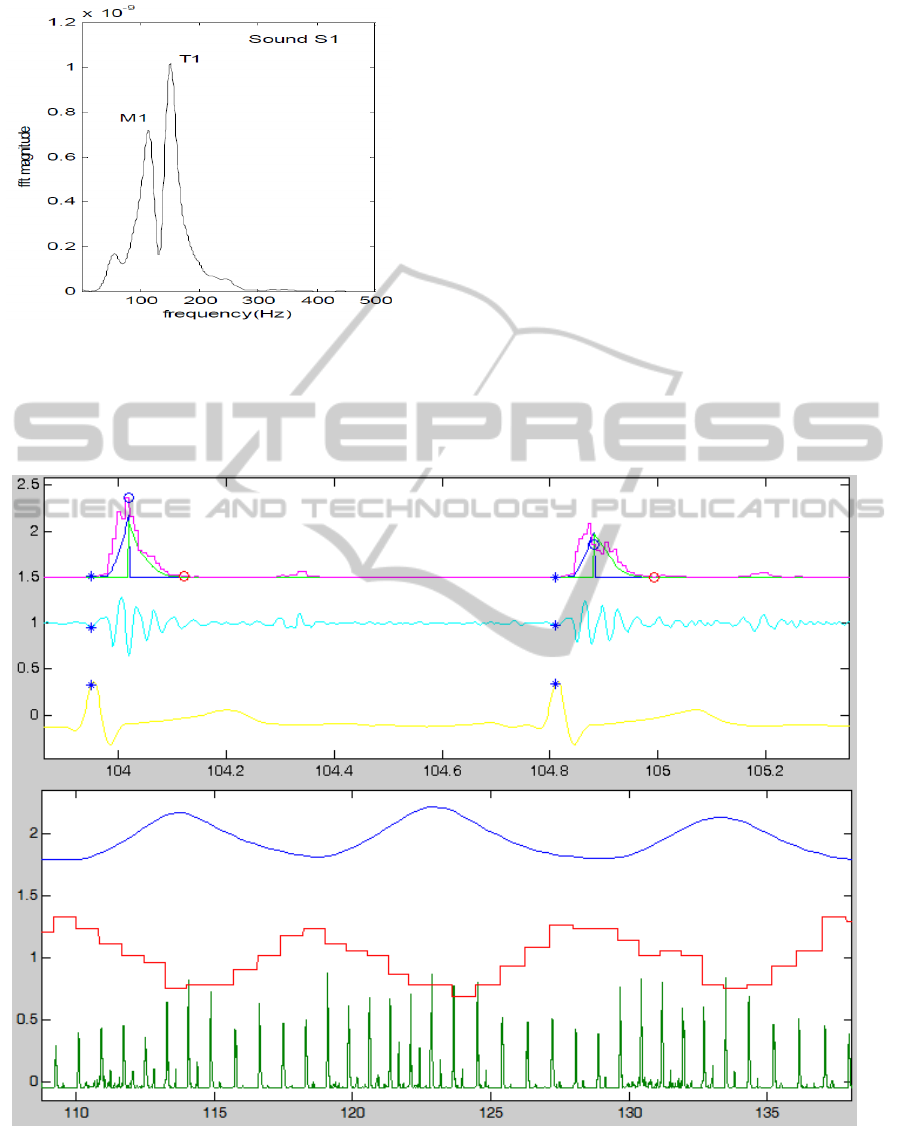
Figure 1: Spectrum of S1 (Debbal and Bereksi-Reguig
2008).
most frequent contributor to their success is robust
and reliable detection of fragments making up
heart sounds. These fragments include FHS, heart
murmurs and extra heart sounds – third and fourth
heart sounds. Pre-processing techniques used
include wavelet transform (Xinpei et al 2009) and
the use of Fourier analysis (El-Segaier 2005).
This study focuses on filtering techniques that
prepare heart sound for the detection of S1 in
an optimal way. The study compares the use of
Fourier analysis and wavelet transform in a number
of bands and decompositions.
2 METHODS
The study presented was performed on 30 volunteers
in good health. During the experiment, the
volunteers were in the supine position. ECG, heart
sound and thorax bioimpedance were measured
continuously. Two types of breathing were
measured; the first was 10–second period breathing
Figure 2: Upper part of the figure: 20-80 Hz envelope (magenta) of the heart sound with integrals (blue, green) representing
gravity center computation, next, heart sound filtered in band 20-80 Hz (cyan) and the last ECG (yellow). Blue asterisk
represent R-wave position, red circle is 20% of R-R interval, blue circle is centre of gravity or S1. The lower part of the
figure represents respiration curve (blue), next R-S1 function (red) and the last one heart sound envelope (green) of
volunteer number 55 during short part of deep breathing. The x-axis represents time in seconds. Time scales differ between
the upper and the lower part of the figure.
FirstHeartSoundDetectionMethods-AComparisonofWaveletTransformandFourierAnalysisinDifferentFrequency
Bands
279
and lasted 5 minutes, it was referred to as deep
breathing. At the end of this exercise, the volunteers
were asked to breathe normally. The second type of
breathing was recorded after 2 minutes of rest. This
type was referred to as spontaneous breathing and
was also recorded for 5 minutes. Spontaneous
breathing records the normal breathing of the
volunteer. The heart sound was recorded using
a microphone held in place by an elastic bandage. It
was measured with a sampling frequency of 500 Hz.
An example of heart sound filtered in the 20–80 Hz
band can be seen as the second curve in the upper
part of Figure 2 coloured cyan. The R-wave was
detected from the ECG signal. It was used as a
reference for S1 detection. Thorax bioimpedance
was filtered with a low-pass filter with a cut-off
frequency at 0.8 Hz. This produces a curve
representing respiration. Impedance was used only
for extracting the respiration curve. The respiration
curve can be seen in the lower part of Figure 2, third
from the bottom, coloured blue.
This study evaluates combinations of filtering
techniques and frequency bands. Stages involved in
filtering techniques evaluation are depicted in Figure
3. At the beginning, heart sound was filtered. The
first type of filtering technique was Fourier analysis.
For this purpose raw heart sound signal was filtered
with a band-pass filter. Filtering was performed in
Matlab environment (MATLAB 2009) by
eliminating frequencies outside of the pass band
using filtfilt function. Transitional parts after
filtering at the beginning and at the end of the signal
were excluded from the signal. As cut-off
frequencies for signal filtering, all combinations of
low cut-off frequencies: 5, 10, 15, 20, 25, 30, 35, 40,
45, 50 Hz and high cut-off frequencies: 10, 15, 20,
25, 30, 35, 40, 45, 50, 60, 80, 100, 120, 150 Hz were
used. A table with all these combinations can be
seen in Figure 4. The upper two tables represent
filtering using Fourier analysis, with a bottom band
cut-off frequency in the leftmost column. The upper
cut-off frequencies are in the first row. For example
band pass filter with low cut-off frequency 20 and
the high cut-off frequency 80 is located in the fifth
row marked with 20 and the twelfth column marked
with 80. The second type of filter used was wavelet
transform in which filter banks from the Daubechies
family, numbers 4 and 14 (db4, db14) were used.
A filter bank from the Coiflet family, number 2
(coif2) was also used. They showed the best results
during the initial phase of this study and were also
evaluated by a previous study (Messer et al 2001).
Wavelet transform decomposed the signal into a 5
level details. Again, Matlab environment (MATLAB
2009) was used for signal decomposition, namely
function swt. The spectrum of the first level detail
corresponds to approximately a band of 125–250
Hz, the second detail level to 62.5–125 Hz, the third
detail level to 31.25–62.5 Hz, the fourth detail level
to 15.5–31 Hz and the fifth detail level to 8–15.5 Hz.
The signal is reconstructed by summing detail
levels. Let
(n),
(n),
(n),
(n) and
(n) be
the detail levels of the original signal
.
Reconstructed signal
is then
(2),
where∈1,5, ∈2,5, . The equation
(2) is the sum of details ranging from the lowest
detail –l to the highest detail –h. Note, that the
highest and the lowest detail can be of the same
level and that the highest detail of the sum is greater
than the lowest. All the combinations from the
equation (2) were used for the signal filtering. These
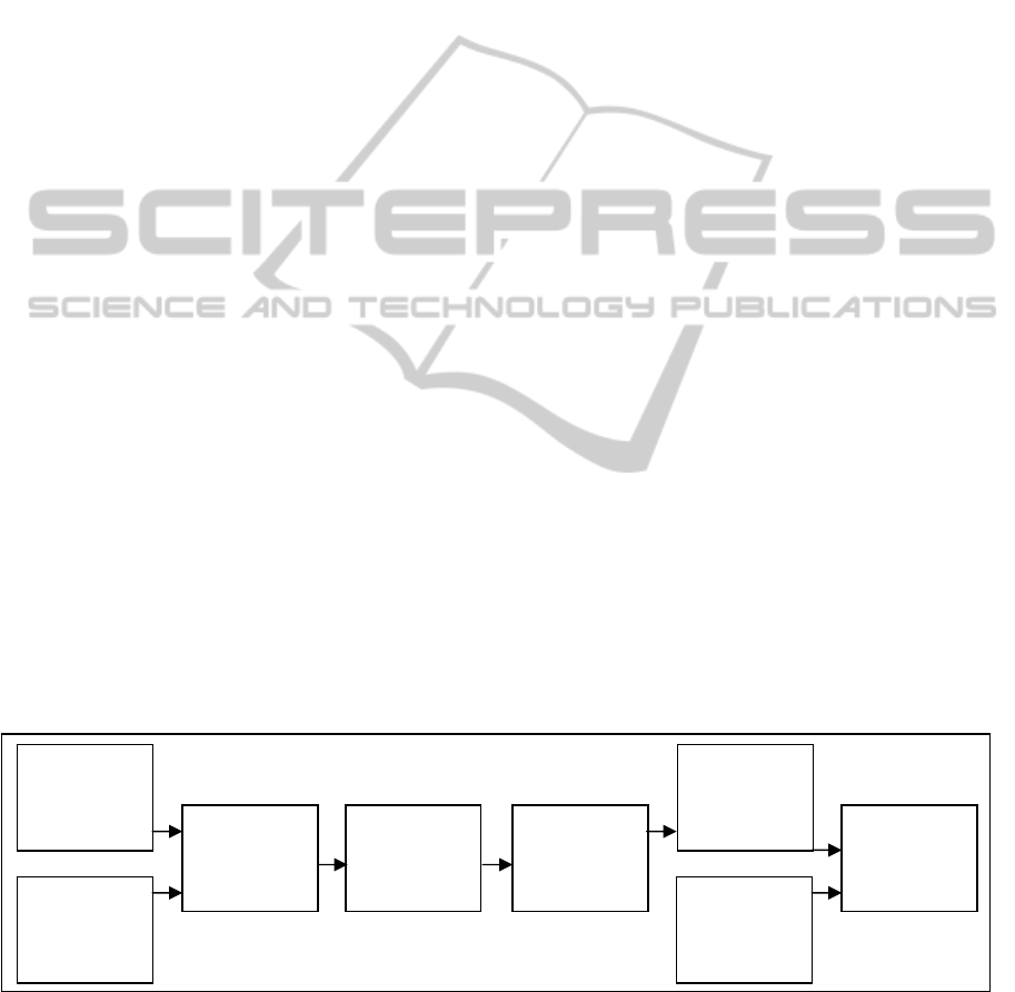
Figure 3: Block diagram with steps involved in comparing filtering techniques. First, heart sound was filtered using Fourier
analysis or wavelet transform. Next, envelope was computed using NASA (normalized average Shannon energy detection
algorithm - equation (3)) and then centre of gravity (S1) of interval starting from R-wave to the R-wave + 20 % of the R-R
distance, abbreviated <R, 0.2R-R>was computed. S1 distance from R-wave was determined for every R-R interval, thus
creating R-S1 function. R-S1 was delayed from 0 to 9 R-R intervals towards respiration and then R-S1 was correlated with
respiration curve.
Fourier
analysis
Wavelet
transform
Envelope
computing
by NASA
Centre of
gravity
computing
R-S1
function
computing
Delay R-S1
by 0 to 9
R-R intervals
Generating
respiration
curve
Correlation
computing
BIOSIGNALS2014-InternationalConferenceonBio-inspiredSystemsandSignalProcessing
280
Subject 32 - Deep breathing - Filtered using Fourier analysis
cut-off
10 15 20 25 30 35 40 45 50 60 80 100 120 150 Hz
5 -0,05 0,32 0,65 0,77 0,86 0,85 0,82 0,83 0,83 0,83 0,83 0,83 0,83 0,83
10 0,64 0,83 0,86 0,89 0,85 0,81 0,81 0,81 0,81 0,81 0,81 0,81 0,81
15 0,48 0,63 0,72 0,66 0,58 0,58 0,58 0,62 0,59 0,58 0,57 0,58
20 0,47 0,52 0,46 0,44 0,46 0,48 0,49 0,49 0,49 0,49 0,49
25 0,12 0,35 0,34 0,37 0,37 0,35 0,38 0,38 0,39 0,39
30 0,28 0,22 0,3 0,4 0,45 0,44 0,44 0,44 0,45
35 0,43 0,53 0,6 0,65 0,69 0,69 0,7 0,7
40 0,44 0,46 0,51 0,61 0,6 0,6 0,6
45 0,29 0,39 0,39 0,38 0,38 0,37
50 0,45 0,45 0,44 0,43 0,45
Hz
Subject 55 - Deep breathing - Filtered using Fourier analysis
cut-off 10 15 20 25 30 35 40 45 50 60 80 100 120 150 Hz
5 0,07 0,17 0,12 0,13 0,13 0,09 0,06 0,06 0,06 0,06 0,06 0,06 0,06 0,06
10 0,13 0,19 0,21 0,14 0,29 0,42 0,45 0,46 0,46 0,46 0,46 0,46 0,46
15 0,44 0,07 0,44 0,54 0,59 0,6 0,61 0,62 0,61 0,61 0,61 0,61
20 0,39 0,5 0,59 0,64 0,64 0,63 0,64 0,64 0,64 0,64 0,64
25 0,45 0,56 0,62 0,61 0,61 0,62 0,61 0,61 0,62 0,61
30 0,45 0,54 0,54 0,53 0,52 0,52 0,53 0,53 0,53
35 0,35 0,43 0,37 0,24 0,24 0,24 0,24 0,23
40 0,18 0,12 0,14 0,24 0,22 0,22 0,21
45 0,16 0,24 0,23 0,22 0,22 0,22
50 0,19 0,19 0,2 0,21 0,22
Hz
Wavelet filter, deep breathing Wavelet filter, deep breathing
Subject 32 Subject 55
level
5 4 3 2 1 level 5 4 3 2 1
5
0,02 0,77 0,87 0,87 0,87
5
0,21 0,2 0,22 0,22 0,22
4
0,77 0,85 0,85 0,85
4
0,26 0,22 0,23 0,23
3
0,21 0,26 0,26
3
0,61 0,64 0,64
2
0,41 0,45
2
0,15 0,15
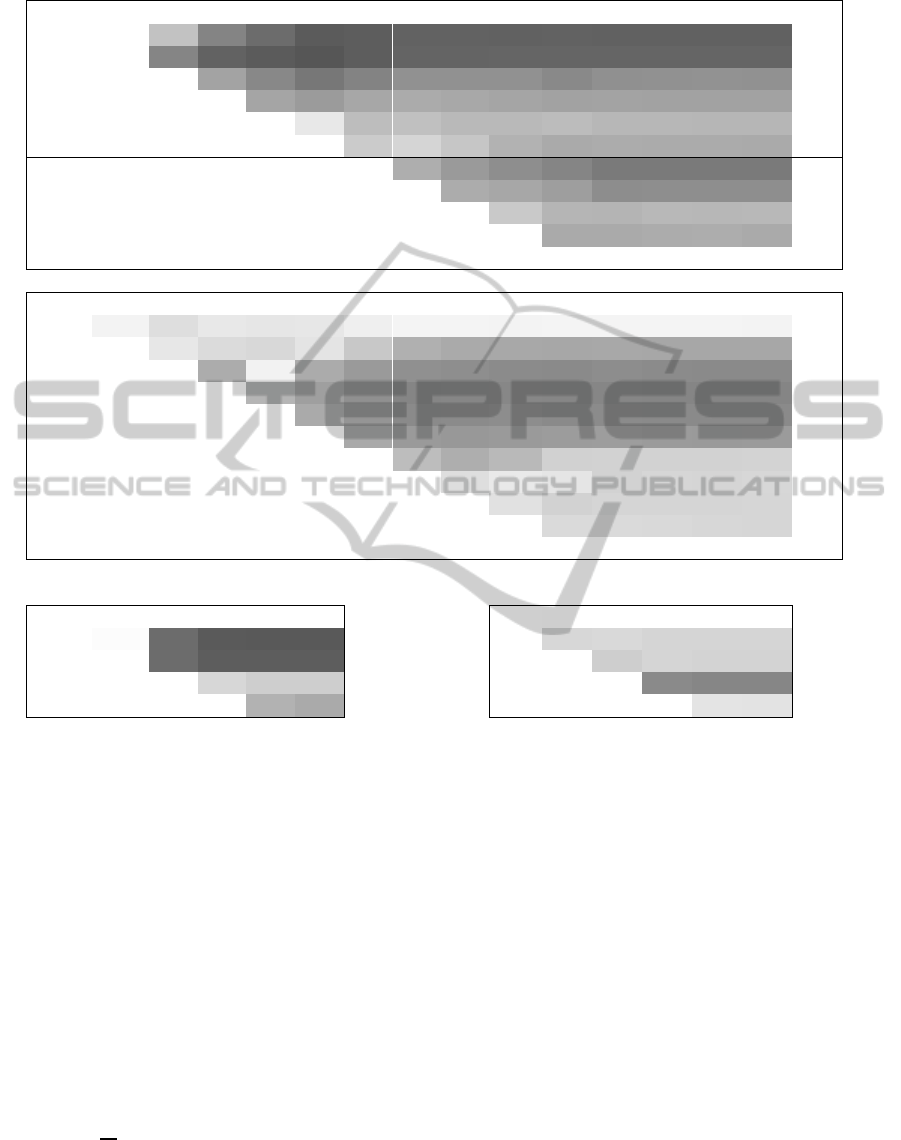
Figure 4: Numbers in the tables represent correlations between R-S1 function and respiration of volunteers number 32 and
55 after heart sound was filtered with a band-pass filter using Fourier analysis with low cut-off frequency from first column
and high cut-off frequency from first row in upper two tables. Lower two tables represent the same correlations after
summing wavelet detail levels ranging from the lowest detail from first column to highest detail from first row.
combinations can be seen in the lower part of Figure
4. For example, the sum of details 5, 4, 3 used for
signal reconstruction are located in row marked with
5 in the table representing the highest detail, and
column marked with 3, representing the lowest
detail used in the sum. Another example, single
detail 2 used for reconstruction, is in row 2 (highest
detail) and in column 2 (the lowest detail of the
sum). After the signal had been filtered, an envelope
was computed using a normalized average Shannon
energy detection algorithm (NASA) (3),
1
|
|
log
|
|
(3)
The envelope of heart sound can be seen as the first
curve in the upper part of Figure 2 and the very
bottom curve in the lower part of Figure 2. The
second one is significantly squeezed, which can be
observed on the x-axis representing time. Next, in
interval starting from R-wave to the R-wave + 20 %
of the R-R distance, abbreviated <R, 0.2R-R>, the
centre of gravity was computed. Computation of the
gravity centre is depicted in Figure 2, the first curve
in the upper part of the figure. Integrals of the
envelope were computed from the left and right side
of the interval <R, 0.2R-R>. Particular integrals are
also depicted in the same place as the envelope with
the blue and green colour. The point at which these
integrals have the same value was found. This point
was declared the centre of gravity and was also S1.
We assume that if S1 was detected correctly then
it should correlate with respiration. For every R-R
interval we computed the mean value of the
FirstHeartSoundDetectionMethods-AComparisonofWaveletTransformandFourierAnalysisinDifferentFrequency
Bands
281
respiration curve and also the R-S1 distance which is
the distance between the R-wave and the detected
S1. The R-S1 function can be seen as the second
curve from the bottom in the lower part of Figure 2.
When we look at the R-S1 function and respiration
in the lower part of Figure 2 it is clear that they are
shifted in respect of each other. Therefore, we
delayed the R-S1 curve towards the respiration curve
in 10 steps, always by one R-R interval. In this way,
we had 10 R-S1 curves, delayed from 0 to 9 R-R
intervals. Next, we computed correlation with all 10
R-S1 functions and R-R segmented respiration curve
as a sign of good or bad detection capability for the
given filter. We found the highest of the 10
correlation coefficients and declared it the
correlation between R-S1 and respiration for the
given filter.
3 RESULTS
We assume that the higher the correlation, the better
the detection of S1. Correlation for spontaneous and
deep breathing was computed separately for each
volunteer. Correlations were entered into the tables
as shown in Figure 4. This figure shows the results
for volunteer number 32 and volunteer number 55
for deep breathing after filtering using Fourier
analysis in the upper part of the figure and after
filtering using wavelet transform at the bottom of the
figure. The values of the correlations are coloured
for better orientation in the tables. Values are
coloured with a grey scale ranging from 1 –darkest
to 0 –white.
Median values - Deep breathing, filtered using Fourier analysis
cut-
off
10 15 20 25 30 35 40 45 50 60 80 100 120 150 Hz
5 0,32 0,44 0,45 0,57 0,54 0,53 0,48 0,46 0,46 0,44 0,43 0,43 0,43 0,43
10 0,39 0,46 0,47 0,4 0,45 0,47 0,46 0,45 0,46 0,45 0,45 0,45 0,45
15 0,44 0,48 0,44 0,46 0,42 0,45 0,44 0,43 0,44 0,44 0,44 0,44
20 0,46 0,46 0,46 0,42 0,45 0,48 0,49 0,48 0,48 0,48 0,48
25 0,37 0,42 0,44 0,48 0,48 0,48 0,52 0,52 0,52 0,52
30 0,36 0,36 0,36 0,42 0,46 0,48 0,49 0,5 0,5
35 0,27 0,38 0,42 0,43 0,46 0,46 0,46 0,46
40 0,31 0,36 0,35 0,36 0,38 0,38 0,38
45 0,24 0,31 0,33 0,37 0,37 0,37
50 0,3 0,3 0,35 0,36 0,36
Hz
Median values - Spontaneous breathing, filtered using Fourier analysis
cut-
off
10 15 20 25 30 35 40 45 50 60 80 100 120 150 Hz
5 0,21 0,2 0,23 0,22 0,23 0,25 0,24 0,24 0,26 0,26 0,26 0,25 0,25 0,25
10 0,25 0,25 0,22 0,24 0,25 0,26 0,23 0,23 0,22 0,22 0,22 0,21 0,21
15 0,27 0,25 0,26 0,33 0,33 0,36 0,36 0,34 0,35 0,34 0,33 0,33
20 0,29 0,31 0,33 0,3 0,25 0,25 0,26 0,27 0,28 0,27 0,27
25 0,31 0,29 0,26 0,27 0,24 0,3 0,31 0,3 0,31 0,31
30 0,25 0,29 0,3 0,25 0,29 0,3 0,3 0,3 0,3
35 0,22 0,25 0,28 0,32 0,33 0,31 0,31 0,31
40 0,21 0,3 0,27 0,21 0,19 0,19 0,19
45 0,23 0,23 0,19 0,21 0,2 0,21
50 0,21 0,26 0,26 0,25 0,25
Hz
Wavelet filter, deep breathing Wavelet filter, spontaneous breathing
Median values Median values
level
5 4 3 2 1 level 5 4 3 2 1
5
0,41 0,45 0,42 0,42 0,42
5
0,25 0,22 0,22 0,22 0,22
4
0,49 0,44 0,45 0,45
4
0,3 0,29 0,3 0,3
3
0,49 0,5 0,5
3
0,28 0,32 0,3
2
0,4 0,38
2
0,29 0,29
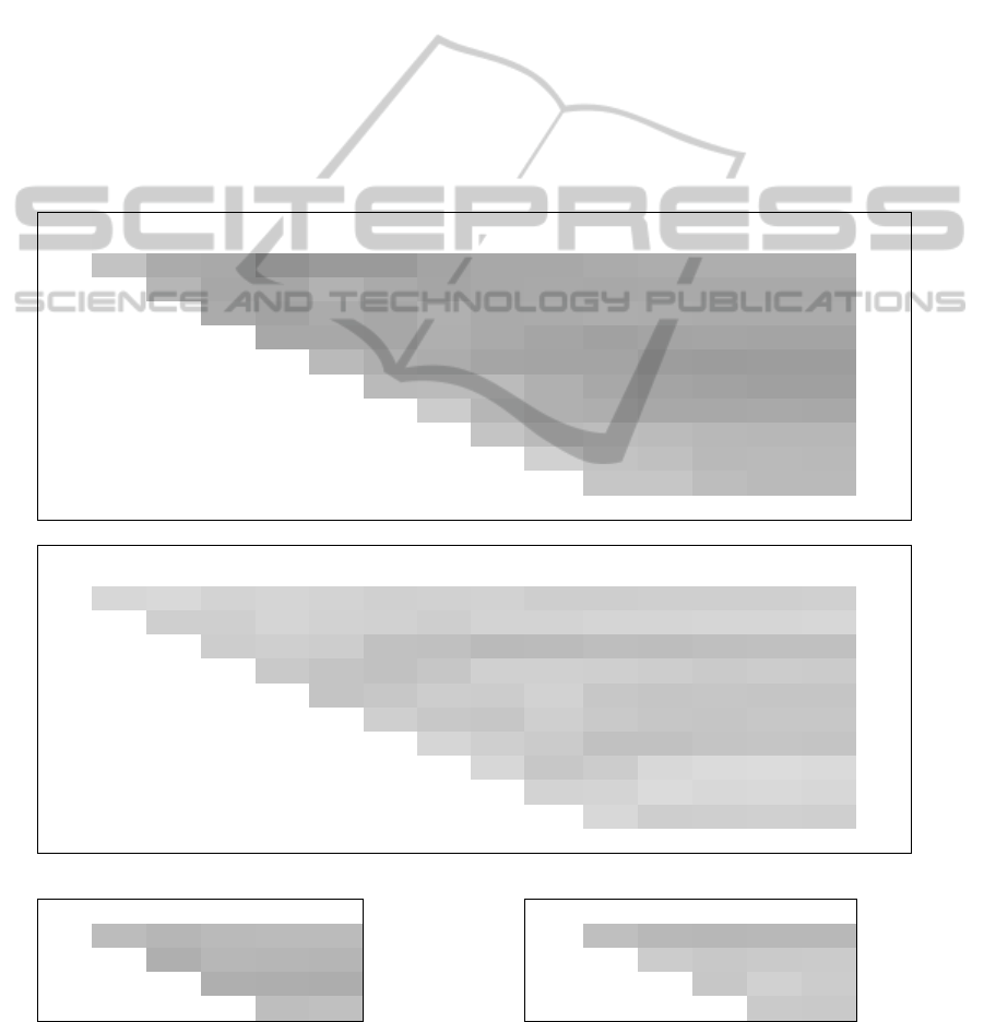
Figure 5: Numbers in the tables represent median correlations between R-S1 function and respiration of all 30 volunteers
after heart sound was filtered with a band-pass filter using Fourier analysis with low cut-off frequency from first column
and high cut-off frequency from first row in upper two tables. Lower two tables represent the same correlations after
summing wavelet detail levels ranging from the lowest detail from first column to highest detail from first row.
BIOSIGNALS2014-InternationalConferenceonBio-inspiredSystemsandSignalProcessing
282

4 CONCLUSIONS
As can be seen in Figure 4, individuals have
different frequency bands in which they correlate
with respiration. This is true for both deep and
spontaneous breathing. As can be seen in Figure 5
median values of correlations do not reach
significantly higher values in any particular areas as
compared to the rest of the table, which strengthens
the claim that the spectrum of S1 that correlates with
breathing is highly individual for each volunteer. We
can say that for each volunteer there is a frequency
band in which heart sound correlates significantly
with breathing. If we compute median of maximum
correlations of all volunteers across all the bands, we
get a median correlation of 0.718 for deep breathing
and 0.585 for spontaneous breathing. We can now
say that R-S1 correlates with respiration for some
filter for each volunteer. Another piece of
information gained from this study is that deep
breathing produces larger values of correlation than
spontaneous breathing. When we compare wavelets
and Fourier analysis, wavelets are not so sensitive in
selecting the optimal band, while the advantage of
Fourier analysis is its capability to tune bands more
precisely. Filter banks db4, db14 and coif2 did not
produce very different results when compared to
each other. On the basis of this study, we can say
that Fourier analysis is sufficient for heart sound
pre-processing. The crucial thing here is appropriate
frequency band selection for each individual.
Computing correlation with respiration proved to be
good sign for correct S1 detection. Further study
would be beneficial for S2 and also for LVET
detection.
ACKNOWLEDGEMENTS
This work was partially supported by grant no.
P102/12/2034 from the Grant Agency of the Czech
Republic and by the European Regional
Development Fund – Projects FNUSA-ICRC
CZ.1.05/1.1.00/02.0123
REFERENCES
Abdelghani D, Fethi B R. 2000. Short-time Fourier
transform analysis of the phonocardiogram signal,
Electronics, Circuits and Systems. ICECS 2000. The
7th IEEE International Conference. 2 : 844–847.
Bernstein D. P., Lemmens H. J., 2005. Stroke volume
equation for impedance cardiography. Medical and
Biological Engineering and Computing, 43 443-50.
Cybulski, G., 2011. Ambulatory Impedance
Cardioagraphy: The Systems and their Applications.
Lecture Notes in Electrical Engineering, ed. Springer.
76, pp 7-37.
Debbal S. M., Bereksi-Reguig F., 2008. Frequency
analysis of the heartbeat sounds. Biomedical Soft
Computing and Human Sciences. 13, 85-90.
El-Segaier M., Lilja O., Lukkarinen S., S-Ornmo L.,
Sepponen R., Pesonen E., 2005. Computer-Based
Detection and Analysis of Heart Sound and
Murmur. Annals of Biomedical Engineering. 33, 937–
942.
JiZhong, Scalzo F., 2013. Automatic Heart Sound Signal
Analysis with Reused Multi-Scale Wavelet
Transform.: International Journal Of Engineering And
Science. 2 50-57.
MATLAB version 7.8.0. 2009a. Natick, Massachusetts:
The MathWorks Inc.
Messer R. S., Agzarian J., Abbott D., 2001. Optimal
wavelet denoising for phonocardiograms. :
Microelectronics Journal. 32. 931-941.
Smith D., Craige E., 1988. Heart Sounds: Toward a
Consensus Regarding their Origin, Am. J. Noninvas.
Cardiol., vol. 2, pp. 169-179.
Xinpei Wang, Yuanyang Li and Churan Sun, Changchun
Liu, 2009. Detection of the First and Second Heart
Sound Using Heart Sound Energy. Biomedical
Engineering and Informatics.
FirstHeartSoundDetectionMethods-AComparisonofWaveletTransformandFourierAnalysisinDifferentFrequency
Bands
283
