Optimal Product Line Pricing for Two Customer Segments with an
Extension to Multi-Segment Case
Udatta S. Palekar, Govind Daruka and Manmeet Singh
Department of Business Administration, University of Illinois at Urbana-Champaign, Illinois, U.S.A.
Keywords:
Pricing, Product Line, Optimization.
Abstract:
In this paper we consider the problem of determining optimal prices for a product line. Items are distinguished
by a single attribute which we call quality and which is proportional to the cost of the item. Demand for an
item is dependent on the price differential between the item and the next item with higher cost. Customers
can be grouped into two segments based on the lowest features acceptable and the maximum acceptable price.
We develop an algorithm to determine the optimal pricing to maximize profit. We also consider assortment
decisions to add or drop items based on regularity conditions and optimality considerations.
1 INTRODUCTION
The existence of consumers with vast heterogeneity
in tastes has made it very common for firms to offer
multiple items with correlated demand, often called a
product line ((Shugan(1984))). A product line is a set
of items that cater to essentially the same customer
need, but that differ from each other due to either the
existence or non-existence of a feature; or variation in
performance with respect to some measure. A prod-
uct line consists of many individual items, which are
referred as variants or items or products. For consis-
tency, we use the term ‘items’ throughout this paper.
(Monroe(1990)) states that within the domain of
pricing strategy, product line price setting is the most
complicated decision area. Product line decisions are
difficult to make because the items in the line are not
usually independent. Substitution patterns of items in
a product line play an important role in this regard.
Some mathematical models for pricing product
lines that take the inter-item dependencies into con-
sideration have been developed like the model by
(Shugan and Desiraju(2001)). The authors assume
that the product line attracts a homogeneous set of
customers where all of them treat the product line as-
sortment alike. But usually, within a product line,
different items attract different classes of customers
based on customer preference. These heterogeneity
among customers can be better modeled by consider-
ing several customer segments.
In this paper, we extend the work of (Shugan and
Desiraju(2001)) to solve the optimal product line pric-
ing problem with multiple customer segments. The
presence of multi-customer segments adds many lev-
els of complexity to the mathematical analysis. First,
we present analysis for two customer segments and
devise an optimal algorithm for pricing. This is then
extended to multiple customer segments. We develop
important managerial insights on the ‘best’ items to
add to a product line and ‘best’ items to drop from a
product line.
2 LITERATURE REVIEW
Marketing literature in the managerially important
area of product line pricing strategies is relatively
sparse due to the interdependencies of the optimal
prices and demand of items in a product line. In
his seminal work on interdependencies in a product
line, (Urban(1969)) develops and tests a mathemati-
cal model encompassing the major factors and market
phenomena affecting the problem of finding the best
marketing mix for a product line. (Palda(1969)) was
amongst the first to consider individual item prices si-
multaneously and his model used interrelated demand
functions. (Little and Shapiro(1980)) were the first re-
searchers to demonstrate the necessity of a nonlinear
sales ‘response’ function in the context of pricing a
product line in supermarkets. Cross-elasticity terms
were explicitly considered while pricing each item in
the line by (Reibstein and Gatignon(1984)). (Lilien
et al.(1992)Lilien, Kotler, and Moorthy) and (Yano
311
S. Palekar U., Daruka G. and Singh M..
Optimal Product Line Pricing for Two Customer Segments with an Extension to Multi-Segment Case.
DOI: 10.5220/0004924303110316
In Proceedings of the 3rd International Conference on Operations Research and Enterprise Systems (ICORES-2014), pages 311-316
ISBN: 978-989-758-017-8
Copyright
c
 2014 SCITEPRESS (Science and Technology Publications, Lda.)

and Dobson(1998))present comprehensive discussion
of marketing models for product line selection.
(Blattberg and Nelsin(1990)), (Levy and
Weitz(2004)), (Shugan(1984)) and (Zenor(1994))
have emphasized the importance of an item’s
price on its item’s profits and the profits of other
items. (Blattberg and Wisniewski(1989)) show
that high-priced brands compete among themselves
and with low-priced brands. Within retail product
lines, high quality/price brands tends to steal sales
from low quality/price brands but converse is not
true ((Mulhern and Leone(1991)), (Sivakumar and
Raj(1997))). Considering these results (Shugan and
Desiraju(2001)) developed a mathematical pricing
model when items exhibit either symmetric or asym-
metric competition and discuss the implications of
asymmetry. They also provide guidelines for changes
in pricing strategies when costs or line composition
changes. (Moorthy(1984)) showed that the effect of
customer self selection leads to competition within
the firm’s own product line such that, the optimal
product and price cannot be determined separately
for each segment. Our work seeks to create such a
methodology that considers product-line pricing in
the context of multiple customer segments.
3 PROBLEM DESCRIPTION
In this paper we consider a vertically differentiated
product line. The demand for any item in the line fol-
lows the distribution function given by (Shugan and
Desiraju(2001)) who consider a product line with V
items and single customer segment. Let i = 1,2,...,V
denote the items which cost the firm c
1
,c
2
,...,c
V
such that c
i
< c
j
for all items i < j. Then the demand
of the i
th
item is given by
D
i
=
{
M (p
i+1
− p
i
) 1 ≤ i < V, p
i
< p
i+1
M (θ − p
i
) i = V, p
i
< θ
(1)
where, p
i
is the price of the i
th
item, M is a mea-
sure of aggregate demand and θ can be interpreted as
the maximum reservation price of the customer seg-
ment of this product line. The reservation price is the
maximum amount any customer is willing to pay.
Since positive demand requires that p
i
< p
j
for
all items i < j they propose a sufficient condition,
which they call regularity condition. Regularity re-
quires: c
i
< A ∀ i = 1,2,...,V , where A is the adjusted
average cost of the line given as
A =
∑
V
k=1
c
k
+ θ
V + 1
(2)
Then the optimal price p
∗
i
for item i is given by p
∗
i
=
i−1
∑
k=0
(A − c
k
), where c
0
= 0.
In this model, an item competes for customers
with the items that are priced immediately above it.
The demand for a particular item along the product
line can then be said to be driven by its price differ-
ence with respect to the next higher priced item.
Next consider two customer segments that are dis-
tinguished by two parameters. First, there is a seg-
ment specific reservation price that limits the items
that customers in that segment can purchase. Second,
each segment has minimum quality/attribute require-
ments that limits from below the items that customers
in that segment are willing to purchase. The poten-
tial consideration set for customers in each segment
is, therefore, bracketed from below and above. The
actual consideration set for each segment, of course,
depends on the prices that the firm sets. Let,
N
1
,N
2
: customer population of the two segments
u
1
,u
2
: index of the lowest acceptable item for the two
segments
H
1
,H
2
: consideration set for the two segments with-
out price
θ
1
,θ
2
: reservation price of the two customer segments
such that θ
2
> θ
1
a: costliest item available to customer segment 1 for
purchase or reservation price boundary item for cus-
tomer segment 1
V
1
= argmax
i=1,V
{c
i
< θ
1
}
Then the potential consideration sets for the two cus-
tomer segments are given by H
1
= {u
1
,...,V
1
} and
H
2
= {u
2
,...,V }.
Consider the most general case in which u
2
< V
1
.
Also let W (a) = {u
1
,...,a} be the set of items that
the firm, through pricing, makes available to segment
1. Then the pricing structure for the product line can
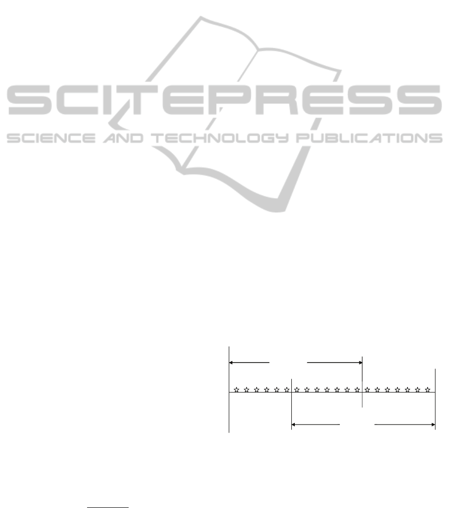
be represented as shown in figure 1.
Customer
Segment 1
Customer
Segment 2
Tier 1
Tier 2
Tier 3
θ
1
θ
2
a
u
2
u
1
1
V
Figure 1: Schematic representation of product line Pricing
for Two Customer Segments .
The solution of the optimal product line pricing
problem breaks up into two parts: the identification
of a; and subsequent pricing given a. Note that in
general u
2
≤ a ≤ V
1
. To obtain a feasible set of prices
ICORES2014-InternationalConferenceonOperationsResearchandEnterpriseSystems
312

for a given a, we require that the regularity condition
is satisfied and the prices are such that the firm’s im-
posed condition that is p
a
< θ
1
and p
a+1
≥ θ
1
is sat-
isfied.
Now supposing that we have identified a, then the
problem of optimally pricing the product line can be
broken down into managing three sets of items con-
sisting of items from 1 to u
2
− 1 attracting customers
from segment 1, items from u
2
to a attracting cus-
tomers from both segments and items from a+1 to
V attracting customers from segment 2. We refer to
these item sets as “tiers”.
The problem reduces to optimally solving three
pricing problems with different boundary conditions
for each tier. Let,
l
1
=
u
2
−
1 be the number of items in tier 1
l
2
= a − u
2
− 1 be the number of items in tier 2
l
3
= V − a be the number of items in tier 3.
Then the adjusted average costs for the tiers are
A
1
=
∑
l
1
k=1
c
k
+ p
u
2
l
1
+ 1
, A
2
=
∑
l
2
k=1
c
k
+ p
a
l
2
+ 1
and A
3
=
∑
l
3
k=1
c
k
+ θ
2
l
3
+ 1
Let Π
i
= (p
i
−c
i
)D
i
denote the profit generated by
the i
th
item in the line, where D
i
, the demand for the
i
th
item is
D
i
=



















M
1
(p
i+1
− p
i
) 1 ≤ i ≤ u
2
− 1
(M
1
+ M
2
) (p
i+1
− p
i
) u
2
≤ i < a
M
1
(θ
1
− p
i
) + M
2
(p
i+1
− p
i
) i = a
M
2
(p
i+1
− p
i
) a < i ≤ V
where, p
V +1
= θ
2
; M
1
= N
1
/(θ
1
− c
u
1
); M
2
=
N
2
/(θ
2
− c
u
2
).
Solving for the optimal prices involves setting the
partial derivative of Π with respect to Π =
∑
Π
i
equal to zero for each of the three segments individu-
ally. The boundary conditions used are: p
0
= c
0
= 0,
p
l
1
+1
= p
u
2
, p
l
2
+1
= p
a
, p
l
3
+1
= p
V +1
= θ
2
. The op-
timal prices obtained are
p
i
=



















iA
1
−
i−1
∑
k=1
c
k
1 ≤ i ≤ l
1
iA
2
−
i−1
∑
k=1
c
k
+
(
l
2
+ 1 − i
l
2
+ 1
)
(p
u
2
− c
u
2
) 1 ≤ i < l
2
iA
3
−
i−1
∑
k=1
c
k
+
(
l
3
+ 1 − i
l
3
+ 1
)
(p
a
− c
a
) 1 ≤ i < l
3
The optimal price of the u
2
item is given as,
p
u
2
=
M
1
M
1
+M
2
(
−
∑
l
1
k=1
c
k
l
1
+1
)
+
c
u
2
l
2
+1
+
∑
l
2
k=1
c
k
l
2
+1
+
p
a
l
2
+1
2 −
M
1
M
1
+M
2
(
l
1
l
1
+1
)
−
l
2
l
2
+1
(3)
For the special case of u
2
= 1, the lowest accept-
able item for the second customer segment is the same
as that of the first customer segment. In this case tier
2 merges with tier 1 and equation (3) need not be eval-
uated.
The optimal price of the a
th
item at the reservation
price boundary is given as,
p
a
=
M
1
θ
1
M
1
+M
2
+ z
1
A
3
+ c
a
z
2
−
∑
l
2
k=1
c
k
l
2
+1
+
(p
u
2
−c
u
2
)
l
2
+1
1 + z
2
−
l
2
l
2
+1
(4)
where z
1
=
M
2
M
1
+ M
2
and z
2
= 1 − z
1
(
l
3
l
3
+ 1
)
Simultaneously solving equation (3) and equation
(4) gives the value of p
a
and p
u
2
, which can then be
used to solve the rest of the prices.
3.1 Optimal Product Line Partition
Thus far, we assumed that the item a, which seg-
ments the product line was known to us. It is clear
though that an appropriate choice of a is required to
maximize product line profits. First we formalize an
intuitive observation, which says that items provide
higher margins when they are limited to the higher
customer segment than when they are made available
to the lower customer segment.
Proposition 1: Assuming regularity conditions,
the price for any item under W (a) will be higher than
under W (a + 1).
Proof: Available from authors.
Consider next any tier t within the product line
with l items having costs c
t
1
,c
t
2
,..., c
t
l
.
Now the optimal price is given as,
p
i
= (iA
t
−
i−1
∑
k=1
c
t
k
) +
(
1 −
i
l
t
+ 1
)
(p
t−1
l
− c
t−1
l
) (5)
The regularity condition p
i+1
− p
i
> 0 gives,
A
t
− c
i
−
(p
t−1
l
− c
t−1
l
)
l
t
+ 1
> 0 (6)
Since c
t
l
is the highest cost item, the regularity condi-
tion can be restated as,
c
t
l
+
(p
t−1
l
− c
t−1
l
)
l
t
+ 1
< A
t
(7)
Therefore, maintaining the regularity condition
implicitly requires that no item cost exceeds the ad-
justed average cost. This puts a constraint on the item
composition of the product line since inclusion and
deletion of items affects the adjusted average cost.
Now, even if the regularity condition is satisfied
and all the items have distinct prices, the firm’s con-
ditions p
a
< θ
1
and θ
1
≤ p
a+1
can get violated due
OptimalProductLinePricingforTwoCustomerSegmentswithan
ExtensiontoMulti-SegmentCase
313

to a linking effect. The condition p
a
< θ
1
is satisfied
if the regularity condition for segment 1 is satisfied
given that ratio of M
1
to M
2
is not very large or very
small. This linking effect and the regularity constraint
imposed over the product line composition makes the
problem hard to solve.
In Proposition 2, we establish that the violation
of the regularity condition for an item composition in
which the firm offers a total of a items to the first cus-
tomer segment implies that the regularity condition
would be violated if any more items are offered to first
segment. This result serves as a stopping criterion for
the search for a.
Proposition 2: If the condition p
a
< θ
1
is violated
for W (a) then corresponding condition ¯p
a+1
< θ
1
will
be violated for W (a + 1).
Proof: Available from authors.
3.2 Optimally Solving the Two Segment
Pricing Problem
We next describe the procedure to determine the opti-
mal item composition.
Procedure:
Step 1: a = u
2
. Solve the pricing problem and
check if the linking condition θ
1
≤ p
a+1
is satisfied.
If not, then let a = a + 1 and solve the new pricing
problem until the linking condition is satisfied giving
a feasible solution. Let the feasible solution is ob-
tained at a = h and z = 1 and the profit is Π(z).
Step 2: Let a = a + 1 and z = z + 1. If regularity
condition is satisfied then resolve the pricing problem
resulting in profit Π(z + 1). Repeat step 2 until regu-
larity condition is violated such that p
a
≥ θ
1
or a =V
1
.
Step 3: Let a = u
2
− 1. This is disjoint segment
scenario. Check if the regularity condition is satis-
fied. If not, let a = a − 1 until the regularity condition
is satisfied. Let z = 0 and z
′
= a. Solve the pricing
problem for such an a giving profit Π(0).
Step 4: Let Z = argmax
z
{Π(z)}. If Z = 0, then
a = z
′
else a = h + Z. Prices of the items are chosen
as per the prices for the item composition with a.
In the case that the two customer segments overlap
the constraint p
u
2
> θ
1
may not to be satisfied. The
profit function can be shown to be strictly concave and
p
u
2
= max{θ
1
, p
∗
u
2
}.
4 COMPUTATIONAL RESULTS
To test the model we collected online retail prices of
items for three different item categories from large na-
tional retail chains in United States. We refer to these
different product line data sets as set 1, set 2 and set
3. The three categories we considered are,
Set 1. Kenmore single room air-conditioners at
Sears.com with six variants,
Set 2. Apple ipods at Bestbuy.com with five vari-
ants, and
Set 3.Kenmore compact refrigerators at Sears.com
with six variants.
First, we estimate the item costs, by randomly se-
lecting a cost within 35% − 45% of the retail price.
We consider two customer segments, assuming that
the population of segment 1 is three times the popu-
lation of segment 2. The values of different param-
eters we use for our pricing model for two customer
segments are shown in Table 1. We assume that first
segment of customers considers all the items for pur-
chase if they are priced within their reservation price
and therefore u
1
= 1 for all the sets. Segment 2 treats
different sets of product line differently and therefore,
u
2
varies from set to set.
Table 1: Base Problem Sets .
Sets 1 2 3
u
1
1 1 1
u
2
2 2 3
θ
1
230 155 195
θ
2
380 275 330
4.1 Pricing Model Performance on Base
Data
To empirically test the performance of our pricing
model in terms of its predictability, we solved each
data set under the test parameters and compare the
prices proposed by our model with respect to current
retail prices. For computational purpose, we assume
that the retailer provides the last two items in each
product line data set exclusively to the second cus-
tomer segment.
Tables 2, 3 and 4 shows the results of applying our
pricing model to the three sets respectively. First col-
umn of the table represents the index of item number.
Second column is the estimate of item costs and the
third column shows the retail prices. Then, we deter-
mine the proposed price, shown in the fourth column
of each table, by solving the pricing problem using
our model.
The last column in each table shows the percent
price difference between the proposed price and the
retail price. These results indicate that the proposed
prices from our pricing model closely resemble the
current trend of retail prices.
ICORES2014-InternationalConferenceonOperationsResearchandEnterpriseSystems
314

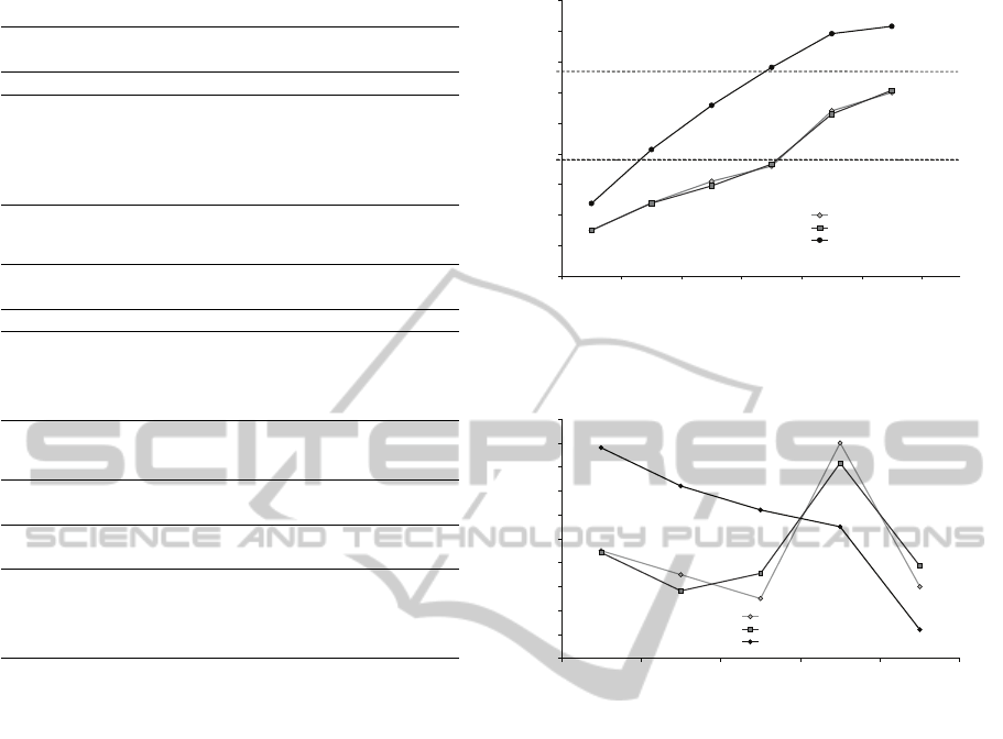
Table 2: Comparison of Prices - Set 1 .
Item Estimated Retail Proposed % Price
Cost Price Price Difference
1 41 99.99 95.11 -4.88
2 61 139.99 149.23 6.60
3 72 189.99 193.74 1.97
4 88 229.99 227.26 -1.19
5 107 299.99 306.84 2.28
6 155 379.99 367.42 -3.31
Table 3: Comparison of Prices - Set 2 .
Item Estimated Retail Proposed % Price
Cost Price Price Difference
1 25 69.99 66.36 -5.18
2 38 99.99 107.72 7.74
3 53 149.99 143.88 -4.08
4 79 199.99 208.25 4.13
5 89 249.99 246.63 -1.35
Table 4: Comparison of Prices - Set 3 .
Item Estimated Retail Proposed % Price
Cost Price Price Difference
1 31 74.98 75.77 1.05
2 47 119.99 120.54 -0.46
3 57 154.99 149.30 -3.67
4 64 179.99 182.40 1.34
5 107 269.99 264.27 -2.12
6 119 299.99 303.13 1.05
Based on our mathematical model, an analysis of
profit by using prices generated from our pricing
model as compared to the store retail prices shows an
increase in profit by 0.5-3 %. The exact increases are
1.196 %, 2.575 % and 0.837 % for data sets 1, 2 and
3 respectively in favor of the prices generated by our
model.
4.2 Comparison with the 1-Segment
Model
We demonstrate the importance of considering two
segments over the single segment model by consider-
ing the prices set 3. We estimate the reservation price
(θ), for a single segment model by satisfying the regu-
larity condition described in equation (2). The result-
ing value is $408.00, which is very high as compared
to θ
2
($330.00), rendering items 4, 5 and 6 beyond
the buying capacity of even the second segment cus-
tomers.
Figure 2 shows this large variation of proposed
prices by the 1-segment model from the retail prices.
Also notice in the figure that for the two segment
model, theproposed prices are very close to the retail
prices and within the reservation price of customers
in segment 2.
0
50
100
150
200
250
300
350
400
450
1 2 3 4 5 6
Product Number
Price ($)
Retail Price
2 Segment Model Proposed Price
1 Segment Model Proposed Price
330$
2
=θ
195$
1
=θ
Figure 2: Two Segment Model Proposed Prices vs One seg-
ment Model Proposed Prices .
0
10
20
30
40
50
60
70
80
90
100
(P
2
-P
1
) (P
3
-P
2
) (P
4
-P
3
) (P
5
-P
4
) (P
6
-P
5
)
Successive Product Pairs
Price Difference ($)
Retail Price Difference
2 Segment Model Price Difference
1 Segment Model Price Difference
Figure 3: Two Segment Model Price gap vs One segment
Model Price gap.
The price difference between successive items is
shown in figure 3. In the 1-segment model, the price
difference between successive items falls steeply. In
the 2-segment model, the price difference does not fall
steeply but has peaks at times when there is a change
in the customer population as the higher segment can
pay more and so this is an intuitively appealing and
more appropriate representation of the market.
5 GENERAL S-CUSTOMER
SEGMENT CASE
In general, the customer population can be divided
into more than two customer segments, say S-
customer segments. The segmentation of customers is
based on the same two measures, namely the lowest
acceptable item and the maximum reservation price.
The total number of tiers formed shall be in the range
of 1 to 2S −1. Since there are more than two customer
segments there is possibility of overlap of many dif-
ferent customer segments. If the lowest acceptable
OptimalProductLinePricingforTwoCustomerSegmentswithan
ExtensiontoMulti-SegmentCase
315

item or reservation price of any two customer seg-
ments are the same, then the total number of tiers
accordingly. Nonetheless, as the number of tiers in-
creases, the complexity of solving the problem also
increases.
The S-segment model can be solved in a man-
ner similar to the 2-segment model by partitioning
the product line into tiers. The mathematical analysis
as done for 2-customer segments is directly extend-
able to the S-customer segments with some general-
ization.Details about this procedure are omitted be-
cause of space. It is important to note that the pro-
cedure is computationally more demanding. How-
ever, the maximum number of computations that may
be needed is
∏
j=1,S−1
(V + 1 − u
j
), giving a worst-case
complexity of O(V
S−1
). However, because of the reg-
ularity condition and the requirement that a
j
≤ a
j+1
, many of these computations will not be needed and
therefore the actual computational burden will be a
lot less. Moreover, the number of customer segments
is unlikely to be very large and so enumerating the
whole problem is computationally not very costly.
REFERENCES
R. C. Blattberg and S.A. Nelsin. Sales Promotion: Con-
cepts, Methods, and Strategies. Engelwood Cliffs NJ:
Prentice-Hall, 1990.
R. C. Blattberg and K.J. Wisniewski. Price induced patterns
of competition. Marketing Science, 8:291–309, 1989.
M. Levy and B.A. Weitz. Retailing Management. Mc Graw
Hill, Inc., 5th edition, 2004.
G. L. Lilien, P. Kotler, and K.S.P. Moorthy. Marketing Mod-
els. Prentice-Hall, N.J., 1992.
J. D. C. Little and J.F. Shapiro. A theory for pricing nonfea-
tured products in supermarkets. Journal of Business,
53(3):199–209, 1980.
K. B. M onroe. Pricing: Making Profitable Decisions. Mc
Graw Hill, Inc., 2nd edition, 1990.
K. S. Moorthy. Market segmentation, self-selection, and
product line design. Marketing Science, 3:288–307,
1984.
F. J. Mulhern and R.P. Leone. Implicit price bundling of
retail products: A multi-product approach to maxi-
mizing store profitability. Journal of Marketing, 55:
63–76, 1991.
K. S. Palda. Economic Analysis for Marketing decisions.
Engelwood Cliffs NJ: Prentice-Hall, 1969.
D. J. Reibstein and H. Gatignon. Optimal product line pric-
ing: The influence of elasticities and cross elasticities.
Journal of Marketing Research, 21:259–267, 1984.
S. M. Shugan. Comments on pricing a product line. Journal
of Business , 57(1):S101–107, 1984.
S. M. Shugan and R. Desiraju. Retail product-line pricing
strategy when costs and products change. Journal of
Retailing, 77:17–38, 2001.
K. Sivakumar and S.P. Raj. Quality tier competetion: How
price change influences brand choice and category
choice. Journal of Marketing, 61:71–84, 1997.
G. L. Urban. A mathematical modelling approach to prod-
uct line decisions. Journal of Marketing Research, 6:
40–47, 1969.
C.A. Yano and G. Dobson. Profit optimizing product line
design, selection and pricing with manufacturing cost
considerations: A survey. In: Ho, T.H. and C.S.
Tang (Eds.), Product Variety Management: Research
Advances. Kluwer Academic Publishers, Dordrecht.,
pages 145–175, 1998.
M. J. Zenor. The profit benefits of category management.
Journal of Marketing Research, 31:202–213, 1994.
ICORES2014-InternationalConferenceonOperationsResearchandEnterpriseSystems
316