
Interest Operator Analysis for Automatic Assessment of Spontaneous
Gestures in Audiometries
A. Fern
´
andez, J. Marey, M. Ortega and M. G. Penedo
Department of Computer Science, VARPA Group, University of A Coru
˜
na, Lab. 0.2, Facultad de Inform
´
atica,
Campus de Elvi
˜
na, 15071, A Coru
˜
na, Spain
Keywords:
Hearing Assesment, Cognitive Decline, Facial Reactions, Optical Flow, Interest Operators.
Abstract:
Hearing loss is a common disease which affects a large percentage of the population. Hearing loss may have
a negative impact on health, social participation, and daily activities, so its diagnosis and monitoring is indeed
important. The audiometric tests related to this diagnosis are constrained when the patient suffers from some
form of cognitive impairment. In these cases, audilogist must try to detect particular facial reactions that
may indicate auditory perception. With the aim of supporting the audiologist in this evaluation, a screening
method that analyzes video sequences and seeks for facial reactions within the eye area was proposed. In
this research, a comprehensive survey of one of the most relevent steps of this methodology is presented. This
survey considers different alternatives for the detection of the interest points and the classsification techniques.
The provided results allow to determine the most suitable configuration for this domain.
1 INTRODUCTION
Hearing loss occurs when the sensitivity to the sounds
normally heard is diminished. It can affect to all
age ranges, however, there is a progressive loss of
sensitivity to hear high frequencies with increasing
age. Considering that population aging is nowadays
a global phenomenom (Davis, 1989) (IMSERSO,
2008) and that the studies of Murlow (Murlow et al.,
1990) and A. Davis (Davis, 1995) point out that hear-
ing loss is the disability more closely related to aging,
the number of elder people with hearing impairment
is increasingly higher.
Hearing plays a key role in the process of “active
aging” (Espmark et al., 2002). Active aging is the
attemp to maximize the physical, mental and social
well-being of our elders. Hearing plays a key role
in the process of active aging. This high impact of
the hearing on the aging process makes necessary to
conduct regular hearing checks if any symptom of de-
creased hearing is noticed.
Pure Tone Audiometry (PTA) is unequivocally de-
scribed as the gold standard for audiological evalua-
tion. Results from pure-tone audiometry are used for
the diagnosis of normal or abnormal hearing sensitiv-
ity, namely, for the assesment of hearing loss. It is
a behavioral test so it may involve some operational
constraints, especially among population with special
needs or disabilities.
In the standard protocol for a pure-tone audiom-
etry the audiologist sends auditory stimuli to the pa-
tient at different frequencies and intensities. The pa-
tient is wearing earphones and the auditory stimuli are
delivered through an audiometer to these earphones.
The patient must indicate somehow (typically by rais-
ing his hand) when he perceives the stimuli. In the
case of patients with cognitive decline or other com-
munication disoders, this protocol becomes unforce-
able, since the interaction audiologist-patient is prac-
tically impossible. Taking in consideration that cogni-
tive decline is highly related to age (and hearing loss
is also related to age), the number of patients with
communication difficulties to be assessed is poten-
tially substantial.
Since a typical interaction question-answer is not
possible, the audiologist focuses his attention on the
patient’s behavior, trying to detect spontaneous re-
actions that can be a signal of perception of the au-
diotory stimuli. These reactions are shown by facial
expression changes, mainly expressed in the eye re-
gion. Typically, changes on the gaze direction or ex-
cessive opening of the eyes could indicate perception
of the auditory stimuli. The interpretation of these
reactions requires broad experience from the audiol-
ogist. The reactions are totally dependent on the pa-
tient, each patient may react differently and even a
221
Fernández A., Marey J., Ortega M. and G. Penedo M..
Interest Operator Analysis for Automatic Assessment of Spontaneous Gestures in Audiometries.
DOI: 10.5220/0004926102210229
In Proceedings of the 6th International Conference on Agents and Artificial Intelligence (ICAART-2014), pages 221-229
ISBN: 978-989-758-015-4
Copyright
c
2014 SCITEPRESS (Science and Technology Publications, Lda.)

same patient may show different reactions at differ-
ent times, since these reactions are completely uncon-
scious. Moreover, although the audiologist has expe-
rience enough, it is a entirely subjective procedure.
This subjectivity greatly limits the reproducibility and
robustness of the measurements performed in differ-
ent sessions or by different experts leading to innacu-
racies in the assessments.
The development of an automatic method capa-
ble of analyzing the patient facial reactions will be
very helpful for assisting the audiologists in the eval-
uation of patients with cognitive decline and, this way,
reducing the imprecisions associated to the subjetiv-
ity of the problem. It is important to clarify at this
point that other techniques aimed at the interpretation
of facial expressions are not applicable in this domain.
Most of these techniques (such as (Happy et al., 2012)
or (Chew et al., 2012)) are focused on the classifi-
cation of the facial expressions into one of the typ-
ical expressions (anger, surprise, happiness, disgust,
etc.). The facial expressions of this particular group
of patients do not directly correspond to any of those
categories. They are specific to each patient, without
following a fixed pattern, and, as commented before,
they can even vary within the same patient.
Some initial researchs have already been devel-
oped in (Fernandez et al., 2013) considering the par-
ticularities of this domain. In this work, one of the
most important steps of this methodology is going to
be addressed in detail: the selection of the interest
points used for the optical flow (whose behavior af-
fects every subsequent step of the methodology). Dif-
ferent interest point detectors are going to be studied
in order to find the most appropriate for this specific
problem.
The remainder of this paper is organized as fol-
lows: Section 2 presents the methodology used as
base for this work and introduces the parts over which
this study will be focussed, Section 3 is devoted to the
experimental results and their interpretation. Finally,
in Section 4 some conclusions and future work ideas
are presented.
2 METHODOLOGY
As depicted in the Introduction, the development
of an automatic solution capable of detecting facial
movements as a response to auditory stimuli could be
very helpful for the audiologists in the evaluation of
patients with cognitive decline. An initial approach
was proposed in (Fernandez et al., 2013), which is
going to be the base for this study. A general scheme
of the original methodology is shown in Fig. 1.
Figure 1: Schematic representation of the methodology.
This method focuses its attention on the eye re-
gion, which has been highlighted by the audiologists
as the most representative for the facial reactions of
these patients. This methodology is addressed in a
global way since movements can occur in any area of
the region. In order to address the problem from a
global viewpoint but having a manageable descriptor,
interest points are going to be used.
Therefore, the first steps of the methodology are
aimed to the location of this particular area. The pro-
posed approach previously locate the face region in
order to reduce the search area, and then locates the
eye region within the face region. Both regions are
located applying the Viola-Jones object detector (Vi-
ola and Jones, 2001), the face by the application of
a cascade provided by the OpenCV tool, and the eye
region with a cascade specifically trained for this re-
gion. Once the eye area is located, the motion estima-
tion begins. To that end, two separated frames are an-
alyzed to determine the movement produced between
them. The motion is estimated by applying the itera-
tive Lucas-Kanade (Lucas and Kanade, 1981) optical
flow method with pyramids (Bouguet, 2000). Once
the motion has been detected, it is characterized based
on several descriptors, this characterization will allow
to apply a classifier which will determine the type of
movement occurred. All these stages are further de-
tailed in (Fernandez et al., 2013).
Since the results of the optical flow depend on
the interest points that the method receives as input,
choosing these interest points is a crucial step, since
the following steps will be highly affected by the re-
sults of this stage of the methodology.
Firstly, it is important to describe the characteris-
tics that define an interest point. Usually, these points
are defined by qualities like: well-defined position
on the image, mathematically well-founded, rich in
terms of local information and stable to global per-
turbations. These properties are assigned regularly to
corners or to locations where the colour of the region
suffers a big change.
Considering this, we want to choose those inter-
est points than can be easily matched by the optical
flow. To select them, an analysis between different
interest point detectors was conducted. Each of these
methods has different foundations, and consequently,
a different way of working, so the results that one pro-
vides can be very different from those provided by the
others. The analysis performed in this work is further
explained in Section 3.
ICAART2014-InternationalConferenceonAgentsandArtificialIntelligence
222
Once the interest points are detected over the
reference image, the application of the optical flow
method will provide the location of these points on
the second image. This means that we obtain a cor-
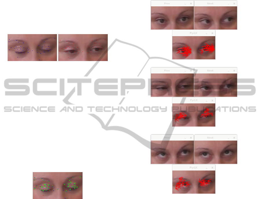
respondence between the two images. In Figure 2 we
can see a sample of this: Fig. 2(a) is the reference im-
age where the detected interest points are represented
in blue, Fig. 2(b) is the second image showing the
correspondence of the interest points obtained by the
optical flow method.
(a) (b)
Figure 2: Sample of the optical flow results: (a) Reference
image with the interest points represented in blue. (b) Sec-
ond image with the corresponding points obtained by the
optical flow represented in red.
With this information, we can build vectors where
the interest point detected on the reference image is
the origin, and the correspoding point on the second
image is the end of the vector. These vectors rep-
resent the direction and the amount of movement of
each point of the reference image. Figure 3 shows the
obtained vectors for the movement between Fig. 2(a)
and Fig. 2(b). Globally, this information is going to
be interpreted as the movement produced for the eye
region between two images.
Figure 3: Movement vectors between Fig. 2(a) and Fig.
2(b).
This representation can be modified into a more
intuive way with vectors depicted as arrows. The
arrow for a particular point represents its movement
from the inicial time considered to the final one. With
this representation it is possible to visually analyze
the results obtained by the optical flow method.
In Figure 4 several samples of this representation
can be observed. Vectors shown in this figure are the
vectors with a length greater than a established thresh-
old (those that represent significant movements), as
they are a good example of how with this technique
it is possible to detect the changes on the eye region.
In Fig. 4(a) the gaze direction is moving towards the
patient’s left, this movement is detected by the optical
flow and represented by the vectors that are poiting to
the right. In Fig. 4(c) the movement is the opposite,
the gaze direction moves slightly to the patient’s right
and the optical flow is still capable of detecting it. In
the case of Fig. 4(b) the eyes open slightly, so in this
case, vector are pointing up following the movement
occurred within the region.
(a)
(b)
(c)
Figure 4: Samples of the movement vectors for different
changes on the eye region: (a) gaze shift to the left, (b) eye
opening and (c) gaze shift to the right.
The obtained vectors are characterized according
to some features, so it is possible to obtain a descrip-
tor that can be classified into one of our considered
movements. After reaching consensus with the ex-
perts, four typical movements were identified as the
most relevant: eye opening, eye closure, gaze shift to
the left or gaze shift to the right. The features used
for obtaining these descriptors are related with the
strength, orientation and dispersion of the movement
vectors, the specific way in which the descriptors are
formed is detailed in (Fernandez et al., 2013). .
As mentioned, the final aim is to classify the
movements produced within this region into one of
the four categories previously mentioned. To that end,
different classifiers have been tested too. The four es-
InterestOperatorAnalysisforAutomaticAssessmentofSpontaneousGesturesinAudiometries
223

tablished classes serve as an initial test set that allow
to draw conclusions about the most suitable interest
operator for this domain. These conclusions will al-
low to establish a foundation for moving forward and
then including new classes that may be deemed rele-
vant by the audiologists. The analysis of the different
alternatives for the classification will be addressed on
the next section.
3 EXPERIMENTAL RESULTS
As commented before, several interest points detec-
tors were tested in order to find the most appropiate
for this domain. The detectors tested are: Harris cor-
ner detector (Harris and Stephens, 1988), Good Fea-
tures to Track (Shi and Tomasi, 1994), SIFT (Lowe,
2004), SURF (Bay et al., 2008), FAST (Rosten and
Drummond, 2005) (Rosten and Drummond, 2006)
and a particular version of Harris with a little modifi-
cation. Also different classification techniques were
tested, in order to find the better detector-classifier
combination.
Video sequences show patients seated in front of
the camera as in Fig. 5. As showed in the picture,
the audiometer is also recorded so the audiologist can
check when he was delivering the stimuli. Video se-
quences are Full HD resolution (1080x1920 pixels)
and 25 FPS (frames per second). Despite the high
resolution of the images, it is important to take into
account that the resolution of the eye region will not
be as optimal, and moreover, lighting conditions will
affect considerably.
Figure 5: Sample of the particular setup of the video se-
quences.
Test were conducted with 9 different video se-
quences, each one from a different patient. Each au-
diometric test takes between 4 and 8 minutes. Con-
sidering that video sequences have a frame rate of
25FPS, an average video sequence of 6 minutes will
have 9000 frames, implying a total number of 81000
frames for the entire video set. Taking into account
that reactions only occur in a timely, we finally have
128 pairs of frames to be considered. Since each eye
is considered separately, the test set will consist of
256 movements. These movements are labeled into
four classes depending in the movement they repre-
sent (see Table 1).
Table 1: Number of samples for each class of movement.
Eye opening Eye closure Gaze left Gaze right
80 82 46 48
Three different experiments were conducted ir or-
der to find the best detector for this domain. The three
experiments are:
1. Find the best classifiers.
2. Find the best configuration parameters for each in-
terest points detector.
3. Evaluate the detector-classifier results.
3.1 Classifier Selection
In this part of the research, different classifiers were
tested with the aim of selecting the three best methods
for applying them on the following tests. The consid-
ered classifiers are provided by the WEKA tool (Hall
et al., 2009), and they are: Naive Bayes, Logistic,
Multilayer Perceptron, Random Committee, Logistic
Model Trees (LMT), Random Tree, Random Forest
and SVM.
To obtain this results, 18 tests were conducted for
each pair detector-classifier, where each one of this
test is a result of a 10-fold cross validation. Comput-
ing the average per method (without considering the
detector used) we obtain the results shown in Figure 6.
As it can be observed on this graph, all the methods
obtain an accuracy between 60 and 75%. Worst re-
sults are observed for Naive Bayes, Logistic and Ran-
dom Tree. Best results are obtained with SVM, fol-
lowed by Random Committee and Random Forest, so
these are going to be the three classifiers considered
for the next survey.
3.2 Adjustment of Parameters
This methodology makes use of different parameters,
that are going to be adjusted according to this experi-
ment. The parameter adjustment is performed depen-
dently on the method used. The parameters studied in
this section are:
• Number of detected points: it indicates the num-
ber of points that the detector needs to select. Very
ICAART2014-InternationalConferenceonAgentsandArtificialIntelligence
224
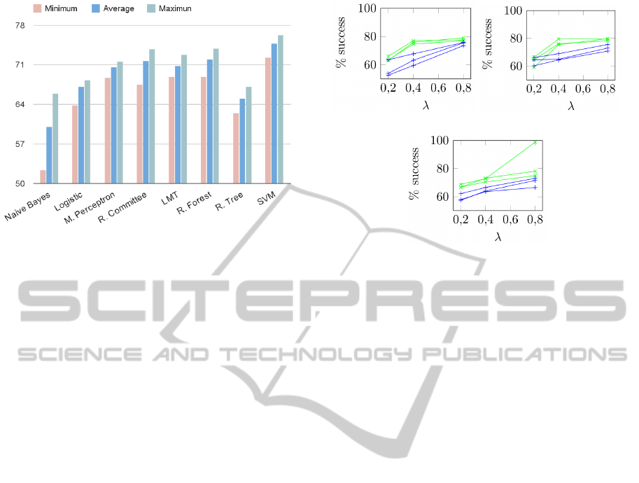
Figure 6: Minimum, maximum and average success per-
centage by classifier.
few points may not be enough to creat a correct
motion descriptor and a number too high may in-
troduce too much noise.
• Minimum percentage of equal points to remove
the movement: sometimes, the detected motion
may be due to global motion between the two
frames and not to a motion within the region. This
will imply a high number of vectors with the same
direction and strength. With the aim of removing
this offset component, the parameter λ is intro-
duced. This parameter indicates the required min-
imum percentage of equal vectors to be consid-
ered a global motion, and consequently, discard
them.
• Minimum length: very short vectors will not be
representative of motion. In order to select the
representative vectors three classes were estab-
lished depending on the length of the vector: u
1
for vectors smaller than 1.5 pixels, u
2
for vectors
between 1.5 and 2.5 pixels and u
3
for vector be-
tween 2.5 and 13 pixels (vectors larger than 13
pixels will be considered erroneous). Vectors in
u
1
are considered too small and are not taked into
account for the descriptor, while vectors in u
3
are
considered relevant and are always part of the de-
scriptors. The inclusion or not of vectors in u
2
is
going to be studied on this section.
3.2.1 Harris
Harris has a particular behavior, it detects few points
concentrated in areas with high contrast. The ob-
tained results are represented in Figure 7. Each line
represents a classifier (Random Committee, Random
Forest and SVM), distinguishing between using only
u
3
vectors (green lines) and u
2
and u
3
vectors (blue
lines).
(a) (b)
(c)
Figure 7: Classification results for Harris. Green lines for
u
3
vectors and blue lines for u
3
and u
2
vectors. Each of the
three lines for each color corresponds to a different classi-
fier. (a) For 40 points of interest. (b) 80 points. (c) 160
points.
It can be observed that, the higher λ is, the better
the results are. Moreover, the inclusion of the vectors
in u
2
shows worse results. It can be noticed that in
Fig. 7(c) there is a velue nearly the 100% of accu-
racy. This value is an outlier that may not be repete-
able, since it breaks the tendency of the other values.
However, it confirms the tendency that with higher λ
values the accuracy increases.
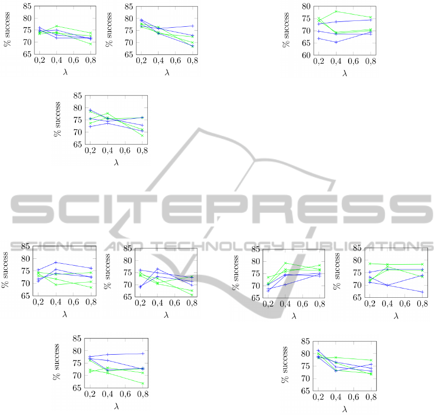
3.2.2 Good Features to Track
This detector was specifically designed for the calcu-
lation of the optical flow. Figure 8 shows the obtained
results for this classifier. As it can be observed, re-
sults are quite consistent regardless of the values of
the parameters. The behavior is better for low values
of λ, and also considering 80 points of interest. Al-
though the results are very similar, including vectors
in u
2
slightly increases the success rate.
3.2.3 SIFT
The SIFT detections are quite similar to the detections
of Good Features to Track. Its results are also broadly
similar (see Fig. 9). Unlike the previous method,
in this case the results for 80 points of interest are
slightly worse than for 40 or 160. The λ parameter
does not affect the results too much. Inclusion of the
intermediate vectors (u
2
) offers also better results.
3.2.4 SURF
SURF detector is a very particular method, since it is
very selective about the detected points. With these
InterestOperatorAnalysisforAutomaticAssessmentofSpontaneousGesturesinAudiometries
225
(a) (b)
(c)
Figure 8: Classification results for Good Features to Track.
Green lines for u
3
vectors and blue lines for u
3
and u
2
vec-
tors. Each of the three lines for each color corresponds to
a different classifier. (a) For 40 points of interest. (b) 80
points. (c) 160 points.
(a) (b)
(c)
Figure 9: Classification results for SIFT. Green lines for u
3
vectors and blue lines for u
3
and u
2
vectors. Each of the
three lines for each color corresponds to a different classi-
fier. (a) For 40 points of interest. (b) 80 points. (c) 160
points.
images, it is not possible to select more than 35-40
points, even with very permissive thresholds. Due
to this particularity, the only results obtained are the
ones shown in Figure 10. Better results are obtained
when including vectors in u
2
, for which the most ap-
propiate value of λ is 0.8.
3.2.5 FAST
The interest points detected by FAST are quite signi-
ficative for this domain. Charts with the results can be
Figure 10: Classification results for SURF. Green lines for
u
3
vectors and blue lines for u
3
and u
2
vectors. Each of the
three lines for each color corresponds to a different classi-
fier.
observed in Fig. 11. Regarding the length of the vec-
tors, results vary according to the number of points
considered. For 40 and 80 points, best results are ob-
tained only considering the strong vectors (u
3
), while
for 160 points best results are obtained when consid-
ering vectors in u
3
and u
2
. For 40 points of interest
the most appropiate is a high value for λ, for 80 points
the results are quite stable regardless of the value of λ,
and for 160 points low values for λ offer better results.
(a) (b)
(c)
Figure 11: Classification results for FAST. Green lines for
u
3
vectors and blue lines for u
3
and u
2
vectors. Each of the
three lines for each color corresponds to a different classi-
fier. (a) For 40 points of interest. (b) 80 points. (c) 160
points.
3.2.6 Harris Modified
The original Harris detector detects few points in ar-
eas with high contrast. To achieve a greater separa-
tion between the points, and therefore more represen-
tative points, a location of the local maximums is con-
ducted. Also a thresholding is applied over the Har-
ris image, and finally, the and operation is computed
with these two images, obtaining this way more dis-
tributed interest points.
Results for this alternative version of Harris are
ICAART2014-InternationalConferenceonAgentsandArtificialIntelligence
226
charted in Fig. 12. These results are similar to the
ones obtained to FAST. In the general case, better re-
sults are obtained considering only vectors in u
3
. For
80 and 160 interest points, the best behavior occurs
for the lower value of λ (0.2). In the case of consider-
ing 40 points, best results occur for λ equal to 0.4.
(a) (b)
(c)
Figure 12: Classification results for Harris modified. Green
lines for u
3
vectors and blue lines for u
3
and u
2
vectors.
Each of the three lines for each color corresponds to a dif-
ferent classifier. (a) For 40 points of interest. (b) 80 points.
(c) 160 points.
3.3 Final Evaluation of the Results
Once the behavior of the different methods in relation
to the configuration of their paremeters has been ana-
lyzed, we are going to compare here the results of the
differents methods with their best configuration. The
optimum configuration parameters and classifiers for
each method are detailed in Table 2.
Table 2: Optimum configuration parameters for each
method.
Method Classifier No. points λ Vectors
Harris SVM 160 0.8 u
3
Good Feat. R. Forest 80 0.2 u
2
& u
3
SIFT SVM 160 0.8 u
2
& u
3
SURF SVM 40 0.4 u
3
FAST R. Forest 160 0.2 u
2
& u
3
Harris mod. SVM 160 0.2 u
3
Results are shown graphically for better under-
standing. In order to assess the capacity of each one
of the interest operators in the detection of the rel-
evant movements the obtained descriptors are com-
pared with the ground truth of movements previously
labeled by the experts.
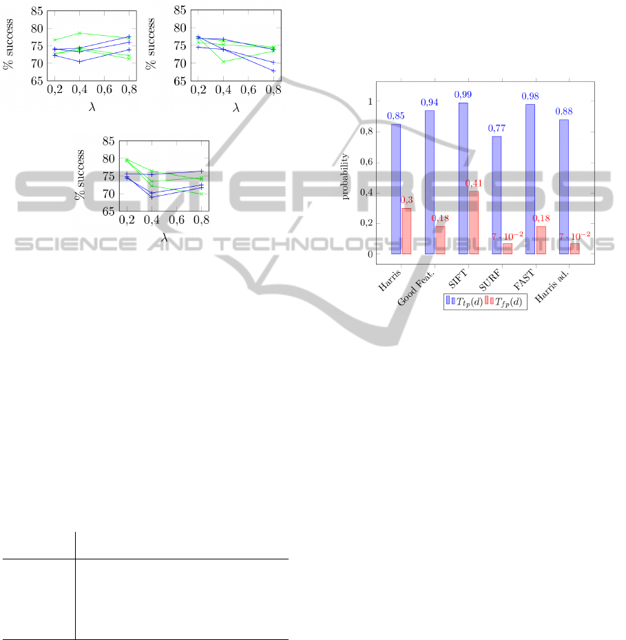
The graph below (Fig. 13) shows the true posi-
tive and false positive rate (T
t p
(d) and T
f p
(d) respec-
tively). It can be note that SURF has a good value
for the false positive rate, but a poor value for the true
positive rate. SIFT is the opposite case, it has a good
value for the T
t p
(d) but poor for the T
f p
(d). The same
happens with Harris, which offers intermediate values
for both rates. Instead, FAST, Good Features to Track
and Harris modified show good values for both rates.
Good Features and FAST offer almost equivalent re-
sults, while Harris modified has a worst T
t p
(d) but it
is compensated with a optimum T
f p
(d) rate.
Figure 13: True positive rate (T
t p
(d)) and false negative rate
(T
f p
(d)) for the different methods.
Given the previous results, only FAST, Good Fea-
tures to Track and Harris modified are considered for
the last evaluation. Figure 14 shows the true positive
rate in detection (T
t p
(d)), the specificity (1 − T
f p
(d))
and the true positive rate in classification (T
t p
(c)). All
the methods have a similar value for the true positive
rate in classification (T
t p
(c)). FAST offers better re-
sults than Good Feature for the three evaluated mea-
sures; so between these two methods, FAST would be
chosen. Comparing between Fast and Harris modi-
fied, it can be observed that the T
t p
(c) is quite similar,
while the T
t p
(d) and the specificity are slightly oppo-
site. FAST offers better results for the T
t p
(d) while
with Harris better results are obtained for the speci-
ficity. The decision of choosing one or another de-
pends on the suitable results for this domain. If we
want to reduce the number of false positives Harris is
the best solution, while if the true positive detections
are more important, FAST is the method that should
be chosen.
4 CONCLUSIONS
A methodology for supporting the audiologists in the
InterestOperatorAnalysisforAutomaticAssessmentofSpontaneousGesturesinAudiometries
227
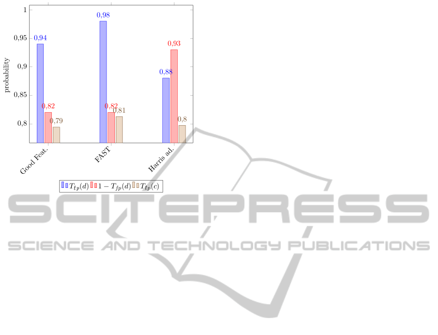
Figure 14: True positive rate (T
t p
(d)) and specificity (1 −
T
t p
(d)) for detection and true positive rate for classification
(T
t p
(c)).
detection of gestural reactions within the eyes region
was developed in previous research, but interest op-
erator analysis for motion detection was not studied
in detail. This paper analyzes different methods for
the selection of the interest points, determines the best
configuration parameters for each one of them, and it
also analyzes its behavior according to different clas-
sifiers. Results obtained with new interest points de-
tectors surpass the previous approach in terms of ac-
curacy.
In clinical terms, the choice of a suitable interest
points detector for this domain may improve the accu-
racy in the detection and interpretation of the gestural
reactions.
Future works will involve an extension of the
training dataset so a robust classifier can be trained
with the configurations established by this work. This
classifier may then by applied over the video se-
quences in order to detect the relevant movements
and, thus, serve to assist the audiologists.
ACKNOWLEDGEMENTS
This research has been partially funded by Ministerio
de Ciencia e Innovacin of the Spanish Government
through the research projects TIN2011-25476.
REFERENCES
Bay, H., Ess, A., Tuytelaars, T., and Van Gool, L. (2008).
Speeded-up robust features (surf). Comput. Vis. Image
Underst., 110(3):346–359.
Bouguet, J.-Y. (2000). Pyramidal implementation of the
Lucas-Kanade feature tracker: Description of the al-
gorithm. Intel Corporation, Microprocessor Research
Labs.
Chew, S., Rana, R., Lucey, P., Lucey, S., and Sridharan, S.
(2012). Sparse temporal representations for facial ex-
pression recognition. In Ho, Y.-S., editor, Advances in
Image and Video Technology, volume 7088 of Lecture
Notes in Computer Science, pages 311–322. Springer
Berlin Heidelberg.
Davis, A. (1989). The prevalence of hearing impairment
and reported hearing disability among adults in great
britain. Int J Epidemiol., 18:911–17.
Davis, A. (1995). Prevalence of hearing impairment. In
Hearing in adults, chapter 3, pages 46–45. London:
Whurr Ltd.
Espmark, A., Rosenhall, U., Erlandsson, S., and Steen, B.
(2002). The two faces of presbiacusia. hearing impair-
ment and psychosocial consequences. Int J Audiol,
42:125–35.
Fernandez, A., Ortega, M., Penedo, M., Cancela, B., and
Gigirey, L. (2013). Automatic eye gesture recogni-
tion in audiometries for patients with cognitive de-
cline. In Image Analysis and Recognition, volume
7950 of Lecture Notes in Computer Science, pages
27–34. Springer Berlin Heidelberg.
Hall, M., Frank, E., Holmes, G., Pfahringer, B., Reutemann,
P., and Witten, I. H. (2009). The WEKA data min-
ing software: An update. SIGKDD Explor. Newsl.,
11(1):10–18.
Happy, S., George, A., and Routray, A. (2012). A real time
facial expression classification system using local bi-
nary patterns. In Intelligent Human Computer Inter-
action (IHCI), 2012 4th International Conference on,
pages 1–5.
Harris, C. and Stephens, M. (1988). A combined corner and
edge detector. In Proceedings of the 4th Alvey Vision
Conference, pages 147–151.
IMSERSO (2008). Las personas mayores en Espaa. In In-
stituto de Mayores y Servicios Sociales.
Lowe, D. G. (2004). Distinctive image features from scale-
invariant keypoints. Int. J. Comput. Vision, 60(2):91–
110.
Lucas, B. D. and Kanade, T. (1981). An iterative image
registration technique with an application to stereo vi-
sion. In Proceedings of the 7th international joint
conference on Artificial intelligence - Volume 2, IJ-
CAI’81, pages 674–679, San Francisco, CA, USA.
Morgan Kaufmann Publishers Inc.
Murlow, C., Aguilar, C., Endicott, J., Velez, R., Tuley, M.,
Charlip, W., and Hill, J. (1990). Asociation between
hearing impairment and the quality of life of elderly
individuals. volume 38, pages 45–50. J Am Geriatr
Soc.
Rosten, E. and Drummond, T. (2005). Fusing points and
lines for high performance tracking. In Computer
Vision, 2005. ICCV 2005. Tenth IEEE International
Conference on, volume 2, pages 1508–1515.
Rosten, E. and Drummond, T. (2006). Machine learning for
high-speed corner detection. In Proceedings of the 9th
ICAART2014-InternationalConferenceonAgentsandArtificialIntelligence
228

European Conference on Computer Vision - Volume
Part I, ECCV’06, pages 430–443, Berlin, Heidelberg.
Springer-Verlag.
Shi, J. and Tomasi, C. (1994). Good features to track. In
Computer Vision and Pattern Recognition, 1994. Pro-
ceedings CVPR ’94., 1994 IEEE Computer Society
Conference on, pages 593–600.
Viola, P. and Jones, M. (2001). Robust real-time object de-
tection. In International Journal of Computer Vision.
InterestOperatorAnalysisforAutomaticAssessmentofSpontaneousGesturesinAudiometries
229
