Enhanced Image Processing Pipeline and Parallel Generation of
Multiscale Tiles for Web-based 3D Rendering of Whole Mouse Brain
Vascular Networks
Jaerock Kwon
Department of Electrical and Computer Engineering, Kettering University, Flint, MI, U.S.A.
Keywords: Brain Vascular Networks, Knife-edge Scanning Microscope, Multi-scale Visualization.
Abstract: Mapping out the complex vascular network in the brain is critical for understanding the transport of oxygen,
nutrition, and signaling molecules. The vascular network can also provide us with clues to the relationship
between neural activity and blood oxygen-related signals. Advanced high-throughput 3D imaging
instruments such as the Knife-Edge Scanning Microscope (KESM) are enabling the imaging of the full
vascular network in small animal brains (e.g., the mouse) at sub-micrometer resolution. The amount of data
per brain (for KESM) is on the order of 2TB, thus it is a major challenge just to visualize it at full
resolution. In this paper, we present an enhanced image processing pipeline for KESM mouse vascular
network data set, and a parallel multi-scale tile generation system for web-based pseudo-3D rendering. The
system allows full navigation of the data set at all resolution scales. We expect our approach to help in
broader dissemination of large-scale, high-resolution 3D microscopy data.
1 INTRODUCTION
The brain is foremost a heavily wired neuronal
network, but there is also an intricate network of
blood vessels that serves as an essential conduit for
oxygen, nutrition, and various signaling molecules.
The vascular network can also provide us with clues
to the relationship between neural activity and blood
oxygen level dependent (BOLD) signals in
functional magnetic resonance imaging (fMRI) or
near infrared spectroscopy (NIRS) signals. Thus,
mapping out the full vascular network in the brain is
an important challenge (Mayerich, Kwon, Sung,
Abbott, Keyser, and Choe, 2011).
Advanced high-throughput 3D imaging
instruments such as the Knife-Edge Scanning
Microscope (KESM) enable the imaging of the full
vascular network in small animal brains (e.g., the
mouse) at sub-micrometer resolution. See Figure 1
for more details. This is sufficient to resolve the
smallest capillaries (Mayerich et al., 2011).
The amount of data produced by KESM imaging
of the mouse brain is on the order of 2TB, thus it is a
major challenge just to visualize it at full resolution.
To address this challenge, the KESM Brain Atlas
(KESMBA) was developed (Chung, Sung,
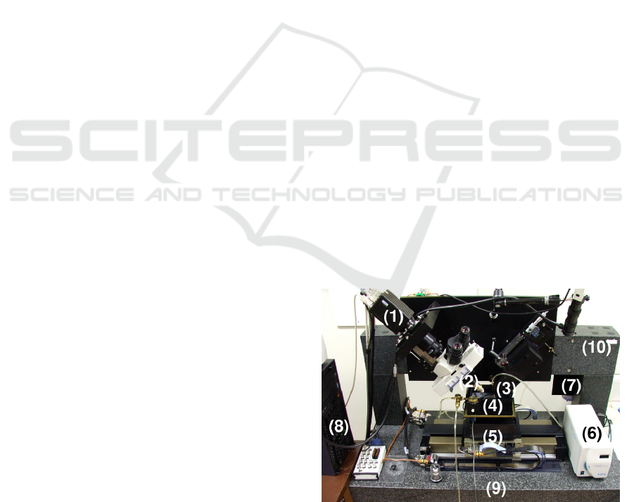
Figure 1: Knife-Edge Scanning Microscope (KESM). (1)
high-speed line-scan camera, (2) microscope objective, (3)
diamond knife assembly and light collimator, (4) specimen
tank (5) three-axis precision stage, (6) white-light
microscope illuminator, (7) water pump for the removal of
sectioned tissue, (8) PC for stage control and image
acquisition, (9) granite base, and (10) granite bridge.
Mayerich, Kwon, Miller, Huffman, Abbott, Keyser,
and Choe, 2011). This system is built on the Google
Maps API, using multi-scale tiles with pseudo-3D
rendering through transparent overlays. Figure 2
shows a screenshot of KESMBA.
783
Kwon J..
Enhanced Image Processing Pipeline and Parallel Generation of Multiscale Tiles for Web-based 3D Rendering of Whole Mouse Brain Vascular
Networks.
DOI: 10.5220/0004926407830789
In Proceedings of the 3rd International Conference on Pattern Recognition Applications and Methods (ICPRAM-2014), pages 783-789
ISBN: 978-989-758-018-5
Copyright
c
2014 SCITEPRESS (Science and Technology Publications, Lda.)
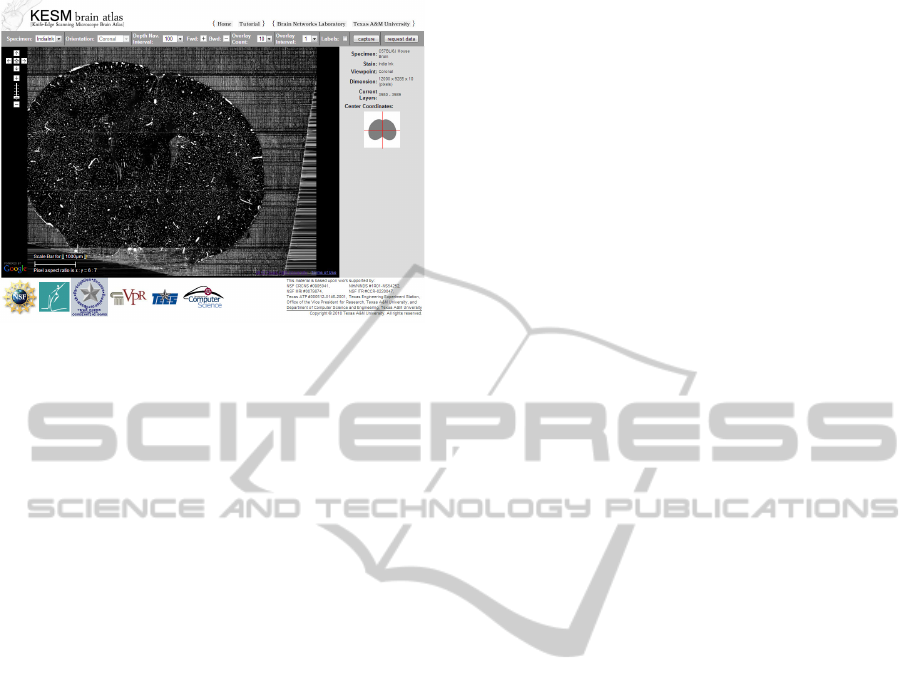
Figure 2: A screenshot of KESM Brain Atlas (KESMBA)
(Chung et al., 2011).
However, the tile generation requires time-
consuming manual calibration and the time required
to download a single visualization is significant (~45
to 55 seconds/page for 20 overlays), requiring a lot
of patience on the part of the user.
To address these two issues, we present an
automated image processing pipeline for KESM
mouse vascular images and a parallel multi-scale tile
generation system for web-based pseudo-3D
rendering that includes pre-overlaid tiles. The
system, built on the OpenLayers API, allows full
navigation and multi-scale viewing of the whole
mouse brain data set at maximum resolution using a
conventional web browser.
2 ENHANCED IMAGE
PROCESSING PIPELINE
KESM employs physical sectioning imaging where
thin slices of tissue are concurrently cut and imaged
(Mayerich, Abbott, and McCormick, 2008). These
slices are then re-assembled in order to produce the
final volumetric data set (Kwon, Mayerich, Choe,
and McCormick, 2008). In this section, we describe
an enhanced image processing pipeline that
performs the following tasks:
The Tissue Area Detector detects the portion
of the raw image that contains actual tissue
data.
The Tissue Area Offset Corrector identifies
and corrects errors in the detected tissue area.
The Cropper crops an image based on the
corrected area information.
The Relighter removes lighting artifacts and
normalizes the inter-image intensity level.
The Merger merges multi-column stacks into
a large, single column image
The Overlay Composer generates pre-
overlaid images with a given number of
images (e.g., an overlay of twenty 1μm-thick
images will give a visualization a 20μm-thick
slab) stack.
The Tiler generates tile images for the web-
based map service
In this paper, we provide details for the Tissue
Area Offset Corrector and the Overlay Composer.
The other phases of the pipeline have been described
previously (Kwon, Mayerich, and Choe, 2011).
Automating the image processing steps is critical
for generating brain atlases since the number of
images is extremely large (e.g. 32,792 images in a
whole mouse brain KESM data set). Previously, we
automated key image processing steps including
noise removal, image intensity normalization, and
tissue area cropping (Kwon et al., 2008) (Kwon et
al., 2011). However, the automation of several
important steps remains, including correction of
tissue area detection results. In addition, we
demonstrate that pre-overlaying of images in the
image stack is necessary to improve page load
performance, and must also be automated.
2.1 Tissue Area Offset Corrector
The image processing pipeline starts from the Tissue
Area Detector. A raw KESM image includes blank
regions flanking the region that contains actual
tissue data. Due to the physical sectioning process,
the precise position of the tissue region in each
image can show some variation due to repositioning
of the knife or the objective during extended
cutting/imaging sessions. We previously describe an
automatic method for detecting the tissue region
based on the right-most edge of the tissue (Kwon et
al., 2011). However some images do not have a clear
boundary due to uneven lighting across the knife
edge. Failure to find a proper tissue boundary leads
to incorrect cropping of the images, which are
difficult to manually correct. Such errors impede
proper reconstruction of 3D geometry in subsequent
stages. However, we find that errors can be detected
by observing the computed tissue region in adjacent
images of the image stack. The sum of the difference
between tissue area offsets in neighboring images is
calculated. A sudden spike indicates an improperly
detected tissue area offset. The summation continues
until it reaches a certain threshold C:
ICPRAM2014-InternationalConferenceonPatternRecognitionApplicationsandMethods
784
N
ni
in
xS until Cx
i
,
(1)
where S
n
is the sum, ∆x
i
= |x(i) − x(i − 1)|, and
x(i) is the tissue area offset of image i. The tissue
area offset x(i) is flagged as a spike (error) when S
n
is less than the minimal chunk size R. A chunk is a
stack of images that are obtained without any
knife/objective repositioning, thus there should be
no variation in x(i). The x(i) difference between two
chunks is expected to be high. Once x(i) is
determined to be a spike, rather than the start of a
new chuck, linear interpolation is applied to the
spike. x(i) will be replaced with x(i − 1). We used C
= 10 and R = 15 in our case for (1). A simple spike
can be removed by the approach described above.
Yet several consecutive and irregular spikes cannot
be removed in a single pass: One more round was
required.
The summation of ∆x
i
continues until it reaches
the maximum number of consecutive spikes (5 in
our case) for the same data set. If the sum of
differences is less than the mini- mum step size for a
new chunk, the set of offsets [x(i), x(i + 1), · · · ] are
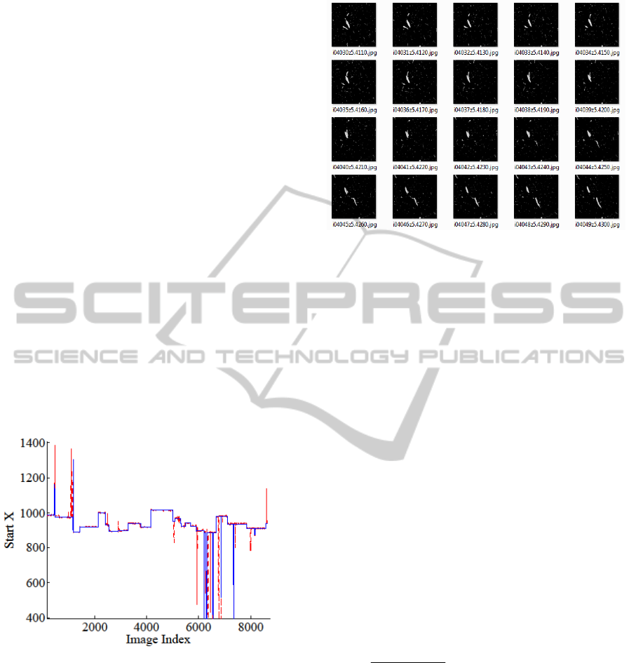
labelled as spikes. Figure 3 shows initial tissue area
offsets compared to the corrected offsets.
Figure 3: Correction of Improperly Detected Tissue
Region. The red dashed lines show the original detection
results. The blue solid lines indicate corrected results.
2.2 Overlay Composer
KESM produces images that represent a 1 mm-thick
tissue section. This allows an unambiguous
geometric reconstruction of the vascular network
(i.e., there are no crossing or overlapping vessel
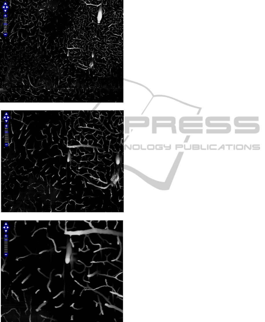
segments in the image). Refer to Figure 4.
However, presenting one image at a time does
not provide insights into the structural organization
of the vascular network (Figure 5 (a)). Overlaying
Figure 4: Series of Thinly Sliced Images. Structural
Organization is hardly seen from a few series of images.
multiple images in the depth direction can overcome
this limitation (Figure 5 (b)). In the current
KESMBA, images with transparent background are
downloaded on-the-fly and composed into an
overlay by the web browser. However, the download
time and overlay computation can be time-
consuming. Furthermore, the addition of the
required alpha channel incurs an extra overhead.
Pre-computing the overlays is an effective
alternative, and in this section we propose an
efficient method that does not require this additional
overhead. We first use (2) to pre-compute multiple
overlays in an image stack:
),,(),(
),,(),(),(
1
1
yxOyxI
yxIyxIyxO
nn
nnnn
(2)
where O
n
(x, y) is an intermediate output image
after composing the n-th and (n + 1)-th image, I
n
(x,
y) is the n-th input image, and the index n = 0 (N - 1)
where N is the number of overlay images. The
attenuation factor α
n
is defined in (3)
q
q
n
s
rns )(
where ,1...0 Nn
(3)
where n is the depth index, N is the maximum
depth, q is the order of the pixel intensity decrease
rate, s is the initial value, and r is the attenuation
rate. The values of the parameters were s = 6, q = 2,
and r = 0.1. Figure 5 (b) shows an example of an
overlay composed of 40 images created using the
above method.
EnhancedImageProcessingPipelineandParallelGenerationofMultiscaleTilesforWeb-based3DRenderingofWhole
MouseBrainVascularNetworks
785
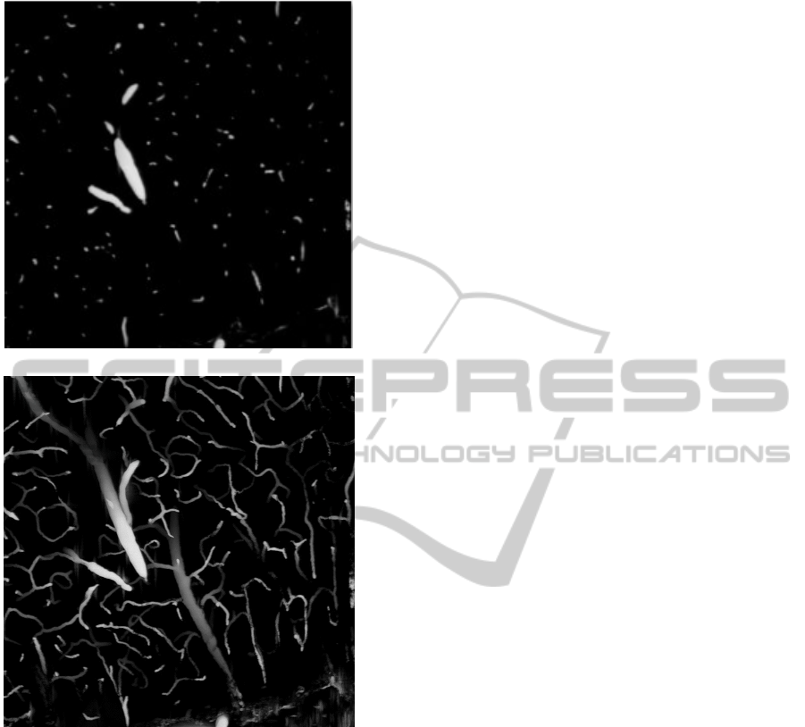
(a)
(b)
Figure 5: Transparent Overlay with Distance Attenuation.
(a) A single KESM image (1 µm thickness). (b) An
overlay of 40 KESM images (40 µm thickness), showing a
local visualization of the vascular network. Objects in the
foreground are brighter and those toward the background
darker (distance attenuation).
3 PARALLELIZATION OF
OVERLAY COMPOSER
Pre-overlaying images can greatly help reduce page
load time for the KESM Brain Atlas, but preparing
the pre-overlaid images (and map tiles) can be very
time consuming. We need to process O(10
4
) very
large images (12,000×9,600) and access more than
100 million pixels with each operation outlined in
the previous section. On average, 1,203ms was
needed to read a single image from a hard drive
directly connected via USB 2.0. It took an average
10,046ms to compose two images to generate an
intermediate overlay. The total time to read and
compose 40 images to produce an intensity
attenuation image was on average
1,203×40+10,046×39 = 439,914ms. The total
number of images of the whole mouse brain
vasculature data set is 9,628, thus it would take
1,177 hours (49 days) to complete the image
composition on a single-core CPU.
Parallelization is a viable option in this case. We
used commodity hardware to parallelize the pre-
computation of overlays, without explicit parallel
programming. The problems that need to be
addressed are as follows: (a) Convenient
deployment of image processing modules that are
being actively developed (i.e., often updated) to all
the workstations. (b) The ability to access the source
data (the KESM image stack) and save the processed
data. (c) Speed loss due to conflicts as more
processes and workstations simultaneously access
shared data resources.
3.1 System Design
To test performance gain due to parallelization, we
designed a system utilizing node-level parallelism
that does not require process-level or thread-level
parallel programming. We built a network of
connected workstations that share a Network
Attached Storage (NAS). We made shared folders in
the NAS and mapped them to network drives on the
workstations so that image processing executables
on the workstations can easily access the data sets.
For data storage, DiskStation DS212j from Synology
was used along with two hard disk drives; 2TB and
3TB. Five workstations were involved in the
experiments. Each workstation had Intel Core i7 920
2.67GHz CPU and 6 GB of triple-channel PC10666
(1,333 MHz) RAM. There are two potential issues
with this setup: (a) concurrent access to storage may
degrade reading and writing performance, and (b)
running multiple concurrent processes on each
workstation can further complicate issue. We test
these factors in the following section.
3.2 System Performance
Each process performs overlay composition. Initially,
we tested the performance with a single process on a
workstation directly attached to the NAS. We then
increased the number of processes to 5, 10, ..., 30,
ICPRAM2014-InternationalConferenceonPatternRecognitionApplicationsandMethods
786
and measured the performance. The number of
workstations was also increased, from 1 to 5. The
performance is measured by the total run time T,
defined in (4).
,
)(
wp
MNtt
T
cr
(4)
Where t
r
is the average time to read an image, t
c
is the average time to compose an overlay of two
images, N is the total number of layers (=40), M is
the total number of images to be processed (=9,628),
and p is the total number of processes. γ and β are
time increment ratios in reading and composing
images respectively as p increases, and w is the
number of involved workstations. The overall
experimental setup is described in Figure 6. Graphs
in Figure 7 show the performance results.
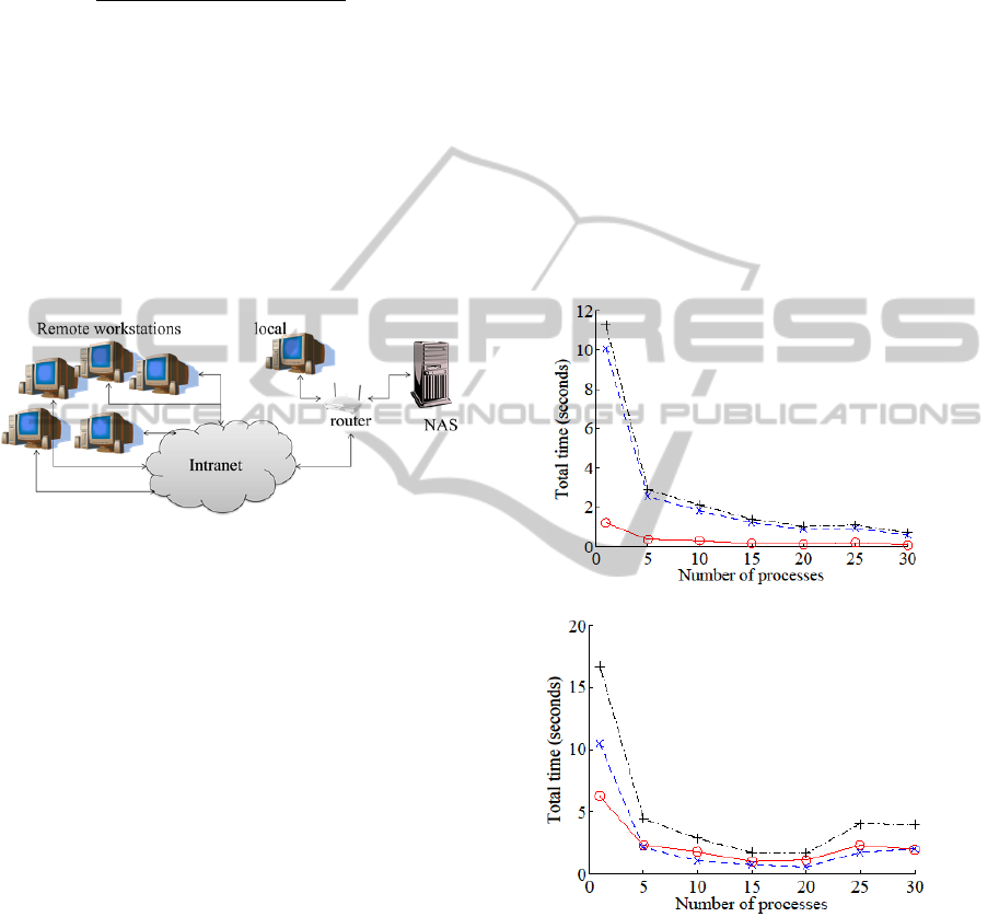
Figure 6: Overall Experimental Setup.
3.2.1 Single Workstation + USB
In this experiment, we varied the number of
processes on a single workstation with the storage
attached via USB. The sum of read time t
r
(o) and
overlay composition time t
c
(×) per process
increased by about three times, but the number of
processors p was increased to 30, so the net
performance gain is 10 times (in terms of reduction
in T: +). We can conclude that using multiple
processes is beneficial when the storage is local and
concurrent access is enabled.
3.2.2 Single Workstation + NAS
We also investigated the case with a single
workstation with a NAS. The results show that read
time t
r
(o) is decreased to the order of time required
to produce the overlay t
c
(×) when the NAS was
accessed in parallel. Total processing time T (+) per
process was increased six-fold, but the number of
processes p increased to 30 so the net performance
gain is 5 times (faster). With max p, the total
processing can be done 10 times faster compared to
the case where a single process is used.
3.2.3 Multiple Workstations (30 Processes)
Here we used up to 3 workstations running 30
processes each. The per workstation computation
time T went up slightly less than two-fold, compared
to the three-fold increase in the number of
workstations w, thus the net reduction in computing
time was 33%.
3.2.3 Multiple Workstations (5 Processes)
Here we used up to 5 workstations with fewer
processes per workstation (=5). In this case, the per-
workstation computing time went up four-fold,
while the number of workstations w increases to five,
distributing the load, thus it lead to a 28% reduction
in computing time.
(a)
(b)
Figure 7: Processing Time. The wall-clock time for
processing a 40-image overlay is shown for different
server/process configurations. (a) Single workstation,
number of process varied, USB-attached storage. (b)
Single workstation, number of process varied, network-
attached storage. (c) Multiple workstations, 30 processes
per workstation, network-attached storage. (d) Multiple
workstations, 5 processes per workstation, network-
attached storage. The results show consistent performance
gain, to a limit, as processes and nodes are added.
EnhancedImageProcessingPipelineandParallelGenerationofMultiscaleTilesforWeb-based3DRenderingofWhole
MouseBrainVascularNetworks
787
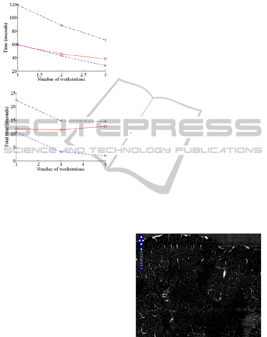
(c)
(d)
Figure 7: Processing Time. The wall-clock time for
processing a 40-image overlay is shown for different
server/process configurations. (a) Single workstation,
number of process varied, USB-attached storage. (b)
Single workstation, number of process varied, network-
attached storage. (c) Multiple workstations, 30 processes
per workstation, network-attached storage. (d) Multiple
workstations, 5 processes per workstation, network-
attached storage. The results show consistent performance
gain, to a limit, as processes and nodes are added. (cont.)
4 ENHANCED KESM BRAIN
ATLAS
To display and navigate the prepared multi-scale
image tiles on a web browser we used OpenLayers,
an open source web service platform. OpenLayers is
an open map API that can display map tiles and
markers. (Refer to http: //openlayers.org for more
details.) The output of our image processing pipeline
is a set of pre-overlaid images that is first converted
into map tile images for OpenLayers.
4.1 Make Map Tiles with GDAL2Tiles
We used GDAL2Tiles to generate map tile images
for OpenLayers. GDAL (Geospatial Data
Abstraction Layer) (http://www.gdal.org) includes
GDAL2Tiles that can generate map tiles for
OpenLayers, Google Maps, Google Earth, and
similar web maps. GDAL can be installed from
OSGeo4W for Windows.
(http://trac.osgeo.org/osgeo4w/). The following
script can be used to create map image tiles from a
single large image.
gdal gdal2tiles.py -p raster -z 0-6 -w
none filename.jpg
We created a script to process all image files in a
folder as follows:
forfiles /m *.jpg /c "cmd /c gdal2tiles
-p raster -z 0-6 -w none @file"
Screenshots of the enhanced KESMBA is shown
in Figure 8. All source code is accessible at
https://github.com/jrkwon/KESMSuite.
5 CONCLUSIONS
In this paper, we presented an enhanced image
processing pipeline for Knife-Edge Scanning
Microscope mouse brain vasculature data. The
pipeline included a Tissue Area Offset Corrector and
Overlay Composer. We also proposed a
parallelization system design and demonstrated its
effectiveness. Finally, we built an OpenLayers-based
web atlas based on the resulting images and tiles.
Our approach is expected to be broadly applicable to
large-scale microscopy data dissemination.
(a)
Figure 8: Enhanced OpenLayers-Based KESM Brain Atlas
Screenshots of the enhanced KESMBA is shown. The
mouse brain vasculature data set is shown at different
scales.
ICPRAM2014-InternationalConferenceonPatternRecognitionApplicationsandMethods
788
(b)
(c)
(d)
Figure 8: Enhanced OpenLayers-Based KESM Brain Atlas
Screenshots of the enhanced KESMBA is shown. The
mouse brain vasculature data set is shown at different
scales. (cont.)
ACKNOWLEDGEMENTS
This publication is based in part on work supported
by Award No. KUSC1-016-04, made by King
Abdullah University of Science and Technology
(KAUST); NIH/NINDS grant #R01-NS54252, NSF
MRI #0079874; and NSF CRCNS #0905041 and
#1208174. We would like to thank B. H. Mc-
Cormick (KESM design), L. C. Abbott (tissue
preparation), J. Keyser (graphics), and B. Mesa
(KESM instrumentation).
REFERENCES
D. Mayerich, J. Kwon, C. Sung, L. C. Abbott, J. Keyser,
and Y. Choe, “Fast macro-scale transmission imiging
of microvascular networks using KESM,” Biomedical
Optics Express, vol. 2, pp. 2888–2896, 2011.
J. R. Chung, C. Sung, D. Mayerich, J. Kwon, D. E. Miller,
T. Huffman, L. C. Abbott, J. Keyser, and Y. Choe,
“Multiscale exploration of mouse brain
microstructures using the knife-edge scanning
microscope brain atlas,” Frontiers in
Neuroinformatics, vol. 5, pp. 29, 2011.
D. Mayerich, L. C. Abbott, and B. H. McCormick, “Knife-
edge scanning microscopy for imaging and
reconstruction of three-dimensional anatomical
structures of the mouse brain,” Journal of Microscopy,
vol. 231, pp. 134–143, 2008.
J. Kwon, D. Mayerich, Y. Choe, and B. H. McCormick,
“Lateral sectioning for knife-edge scanning
microscopy,” in Proceedings of the IEEE
International Symposium on Biomedical Imaging,
2008, pp. 1371–1374.
J. Kwon, D. Mayerich, and Y. Choe, “Automated cropping
and artifact removal for knife-edge scanning
microscopy,” in Proceedings of the IEEE
International Symposium on Biomedical Imaging,
2011, pp. 1366–1369.
EnhancedImageProcessingPipelineandParallelGenerationofMultiscaleTilesforWeb-based3DRenderingofWhole
MouseBrainVascularNetworks
789
