Toward Moving Objects Detection in 3D-Lidar and Camera Data
Clement Deymier and Thierry Chateau
Lasmea-UMR-CNRS 6602, Campus des Cezeaux, 24 Avenue des Landais, 63177 Aubiere Cedex, France
Keywords:
Moving Objects Detection, Photo-consistency.
Abstract:
In this paper, we propose a major improvement of an algorithm named IPCC (Clement Deymier, 2013a)
for Iterative Photo Consistency-Check. His goal is to detect a posteriori moving objects in both camera and
rangefinder data. The range data may be provided by different sensors such as: Velodyne, Riegl or Kinect with
no distinction. The main idea is to consider that range data acquired on static objects are photo-consistent, they
have the same color and texture in all the camera images, but range data acquired on moving object are not
photo-consistent. The central matter is to take into account that range sensor and camera are not synchronous,
so what is seen in camera is not what range sensors acquire. This work propose to estimate photo-consistency
of range data by using his 3D neighborhood as a texture descriptor wich is a major improvement of the original
method based on texture patches. A Gaussian mixture method has been developed to deal with occluded
background. Moreover, we will see how to remove non photo-consistent range data from the scene by an
erosion process and how to repair images by inpainting. Finally, experiments will show the relevance of the
proposed method in terms of both accuracy and computation time.
1 INTRODUCTION
Sequences using sensors such as panoramic range
finders (Lidar, Velodyne, Riegl) or depth camera
(Kinect, SwissRanger) are increasingly common. The
main use of these data is to be realigned in a com-
mon reference thanks to a localization system to form
a coherent point cloud. For this step, ICP (Iterative
Closest Point) algorithm is often used (Rusinkiewicz
and Levoy, 2001), but sometimes this processing re-
quires the help of others sensors. It is indeed usual
to perform this transformation with the assistance
of an inertial unit coupled to a GPS or with a vi-
sual SLAM (Simultaneous Localization And Map-
ping) (Royer et al., 2007). When the 3D point cloud is
realigned, it can be used for navigation of autonomous
robots, but also for mapping and point based 3D ren-
dering of a scene. However, in some applications
such as mobile robotics exploration, we need to de-
tect and remove the moving objects from these data
in order to realize a digital map modeling. To this
end, several methods have been developed based on
the probability of occupancy using only range data.
More precisely, it is important to know if a point
in space is contained within a solid object or is an
empty space (air). This topic is very popular and of-
ten used in moving objects detection (Himmelsbach,
2008; Wurm et al., 2010; Clement Deymier, 2013b).
In fact, an object is moving if measures on his sur-
face are part of a space that is empty at a previous (or
future) time. However, it is unnecessary to know the
occupancy probability at any position but only those
corresponding to impact points (measurements). This
way, it is possible to “filter” moving objects within
the data by measuring the occupancy probability cal-
culated for a detection. If a given measurement has a
low probability then it is very likely that the detection
have been taken on a moving object.
On the other hand, the computer vision commu-
nity works on moving object detection in cameras.
There are many ways to find moving objects in a se-
quence captured by a mobile camera. One of them is
to compute the optical flow or dense matching (Jung
and Sukhatme, 2004) and analyze the results by a mo-
tion segmentation algorithm (Zografos et al., 2010).
Another way is to use a classification algorithm with
a large knowledge database applied to each image,
or even deformable contour approach (Yilmaz et al.,
2004). Unfortunately, all these solutions make strong
hypothesis on the moving object or the scene. Their
movement must be small, they cannot be static for a
while, they cannot be deformable. . . So a pure 3D ap-
proach cannot remove an object from the camera, and
a camera approach cannot help us analyze the range
data because, in this paper, range data are considered
not synchronous with the images.
809
Deymier C. and Chateau T..
Toward Moving Objects Detection in 3D-Lidar and Camera Data.
DOI: 10.5220/0004928608090816
In Proceedings of the 3rd International Conference on Pattern Recognition Applications and Methods (USA-2014), pages 809-816
ISBN: 978-989-758-018-5
Copyright
c
 2014 SCITEPRESS (Science and Technology Publications, Lda.)

Our motivation is to unify the range finding
and camera methods within a global solution named
IPCC (Clement Deymier, 2013a). This one is able
to detect moving objects a posteriori on a sequence
of range data with a color camera by exploiting a
photo-consistency criterion. After the application of
this method, the moving objects are detected in both
camera and range data. Moreover it is possible to re-
store the background in the images where there was
an moving object.
This paper propose a major improvement of the
original version of the algorithm by using a new es-
timation principle of the photo-consistency and new
approach to inpaint image data. Section 2 presents
the principle of the method and focuses on photo-
consistency estimation, scene erosion and image in-
painting. The benefit of the proposed method is ana-
lyzed and discussed in details in section 3 and shows
the relevance of this solution in experimentations.
2 PRINCIPLE OF THE IPCC
ALGORITHM
2.1 A Global Presentation of the
Method
Our algorithm takes in entry two types of data: P
.
=
{P
j
}
j=1,..,n
a set of 3D points coming from range
finder sensor expressed in a common reference, I
.
=
{I
k
}
k=1,..,n
the set of color images provided by one or
more camera, and Ω
k
the projection function in the
image I
k
.
Because range finder acquires measure on object
surface, it’s possible to estimate a photo-consistency
criterion. If this 3D point is seen in more than one
images, the color of each re-projection can be com-
pared and a score of photo-consistency can be cal-
culated and used to classify moving objects. So, the
first step of the IPCC algorithm is to determine which
points are visible or not in the images I
k
.
To this end, a clipping method (2.2) is applied
to determine which points are in the I
k
camera field.
Then, all the visible points are projected in a z-buffer
by disk-splatting to estimate the occlusion constrain
over the scene. Then, all the generated z-buffers
are used to build an occurrence list, which maps 3D
points P
k
to the images where they are seen (2.4).
The second phase is to compute a photo-
consistency criterion. Unfortunately, the pixels color
standard deviation used by (Slabaugh et al., 2003) of
a projected 3D point is not robust and is very sensi-
ble to noise. Usually, to avoid this problem, a rect-
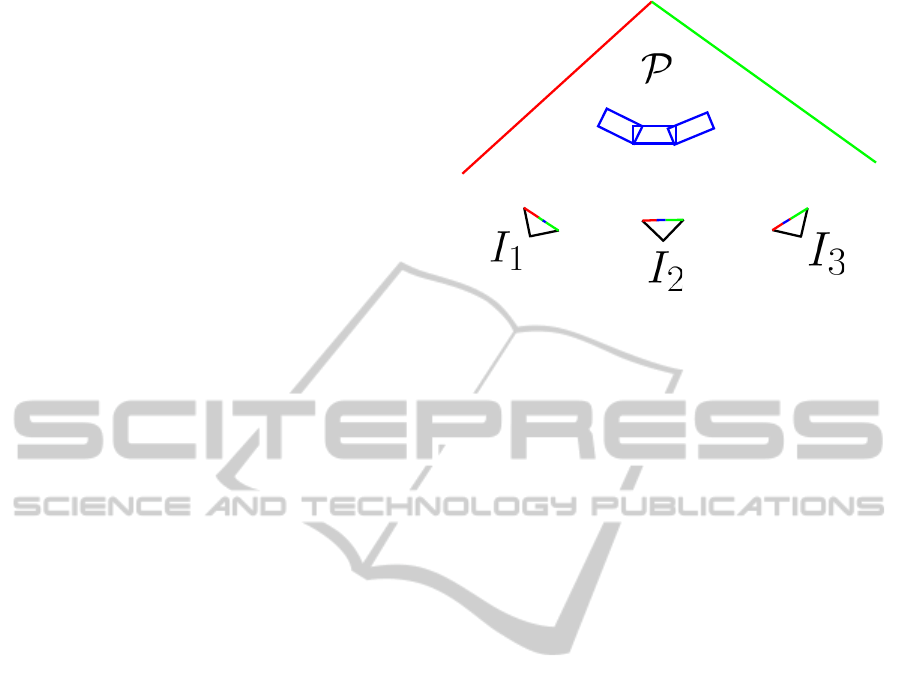
Figure 1: This is a top view of a scene. The 3D point cloud
P is constituted by a green wall, a red wall and a blue car.
The blue car is moving and have been scanned three times
by the range finder sensor. Three images I
1
I
2
and I
3
come
from a camera. Colors of 3D points are given only as indi-
cation but are not known at this step.
angular patch is taken tangent to the 3D surface and
projected in images. The corresponding quadrilater-
als in images are compared by a ZNCC computation
(Zeng et al., 2005). By this way, the system is more
robust and takes more information in account. But,
the IPCC algorithm takes the point cloud of an en-
tire sequence in entry, with the moving object, so, the
surfaces in not differentiable : the normal vector can-
not be computed. To this end, the 3D neighborhood
of a 3D point will be used as a local descriptor (2.5)
by projecting it in the images and getting the corre-
sponding pixels color vector. By this way, the normal
is not needed, no assumption are done on the surface
regularity and the descriptor is invariant to rotation,
translation, scale and projection.
The main difficulty lies in that moving objects are
present in images, so even static objects have a bad
photo-consistency score when moving object get in
front. To deal with this problem, color vectors are
compared with a robust Gaussian mixture and a prin-
cipal mode extraction to obtain the photo-consistency
score (2.5). Then a threshold is used to classify mov-
ing objects and all the corresponding 3D points are
deleted from the scene.
All this steps are computed iteratively until all the
remaining 3D points are photo-consistent. For a bet-
ter understanding of the algorithm, a simple example
will be used to illustrate each step (figure 1). When
the algorithm ends, the photo-consistent point are re-
projected in all images to detect where there was a
moving object. We can optionally chose to highlight
moving object or restore the image background by in-
painting. This part is developed and explained in de-
tail in the subsection 2.7.
ICPRAM2014-InternationalConferenceonPatternRecognitionApplicationsandMethods
810

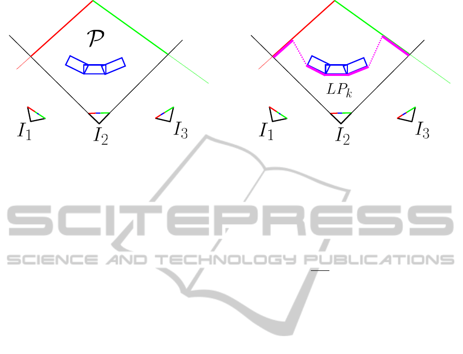
Figure 2: An application of the clipping algorithm to image
I
2
. Dashed lines are outside frustum.
2.2 Image Clipping
This first step consist to find out which 3D points are
inside the camera field of each image I
k
. This phase
is named clipping or frustum culling and needs a lot
of computation time. In fact, if the scene contains ten
million points, and if the camera took one hundred
images, we need to make one billion projections. To
solve this problem, an octree is used to speed-up clip-
ping. After all 3D points have been inserted inside the
octree leaves, the solution given by (Fujimoto et al.,
2012), which consist to compute the intersection be-
tween the camera frustum (four planes) and the oc-
tree cubic node, is used. If a node is intersected by
a camera frustum plane, then the child nodes are ex-
plored. If the node center projected with Ω
k
in the
image I
k
is inside the image, then the child nodes are
explored. At the end, the algorithm returns a leaves
list N
k
which contains all the octree nodes seen in the
k-th images. Figure 2 shows an example of clipping.
2.3 Z-buffer Computation
Once the clipping is done, we need to determine the
occlusion culling for each camera pose (for each im-
age), ie. which object is hidden by another. Oc-
clusion culling is very important because only points
which are really visible in a camera can have a photo-
consistency score. For our method, we need a pes-
simistic depth-buffer because if we see something
through an solid object, this point will be non-photo-
consistent and removed instantly, so we need to be
careful. Moreover, the surface is not differentiable be-
cause of presence of moving object at different time,
so it’s forbidden to try to compute normal vector to
the surface. To avoid normal estimation, we use a Z-
buffer with a disk-splatting algorithm.
For an image I
k
the process is quite simple. We
Figure 3: An example of Z-buffer for the image I
2
. The
point under the pink line are selected by this phase.
initialize a depth image Z
k
with the same size as I
k
.
For all the points P
j
contained in N
k
obtained during
the clipping step the coordinates of the projected point
are computed by : (u
j
, v
j
) = Ω
k
(P
j
). If P
j
have a
depth inferior to the value of Z
k
(u
j
, v
j
) then draw a
disk centered on (u
j
, v
j
) with the same depth value as
P
j
and a radius of
ρ× f
depth
where f is the focal length of
the camera. At the end, return the list of points LP
k
corresponding to 3D points P
j
with a depth inferior or
equal to Z
k
((u
j
, v
j
)).
ρ is the metric size of the disk in the disk-splatting
algorithm. Its value is chosen to fit with the density
of the acquired range data to avoid holes in an object
or a wall The result on example scene can be seen in
figures 3.
2.4 Occurrence Retrieval
For each image, a list LP
k
of visible 3D points is
given by the Z-buffer. In order to estimate the photo-
consistency of the scene, we need to know in which
images a 3D point is seen. This is the role of the oc-
currence list O
.
= {O
j
}
j=1,..,n
where O
j
is a list of all
images containing the point P
j
. To build this struc-
ture, the lists LP
k
are concatenated in an array and
sorted by point index. Then, the occurrences of the
same point number in multiple views are regrouped
in O
j
and sent to the photo-consistency estimation.
2.5 Photo-consistency Estimation
In this part, to simplify index and formula, the photo-
consistency estimation will be explained for one 3D
point call P
j
. The same computation is assumed to
be done on all the points visible in a minimum of 3
images (ie. size(O
j
) ≥ 3)
TowardMovingObjectsDetectionin3D-LidarandCameraData
811

2.5.1 Building the Neighborhood Set V
As we said previously, the 3D neighborhood of a point
P
j
will be used as local texture descriptor to com-
pute the photo-consistency score of the point P
j
. Let
V
k
∈ V the 3D neighborhood of the point P
j
among
the 3D points visible in the view I
k
∈ O
j
. So for a
3D points P
j
for each view I
k
, we are looking for 3D
points visible (ie. ∈ LP
k
) in this view and in a neigh-
borhood of radius σ centered in P
j
. This step is done
by searching in the list of visible points in a view I
k
which is exactly the list provided by the z-buffer :
LP
k
. The free parameter σ determine the 3D sphere
where we consider constant the probability density of
being a moving object. It is chosen empirical to fit
the approximative minimal size of an moving object
(usually σ = 0.15m).
2.5.2 Extracting Color Vector Descriptor Set C
In a second step, for each V
k
∈ V , the 3D points in this
neighborhood are projected in the corresponding im-
age I
k
by Ω
k
to obtain a color value (via a bi-cubic
interpolation) to build a descriptor color vector C
k
.
The color vector C
k
contains for each 3D points of
the neighborhood V
k
a color value given by the im-
age I
k
. Now, we get a set of texture descriptor for a
considered point P
j
: C
.
= {C
k
}
j=1,..,n
.
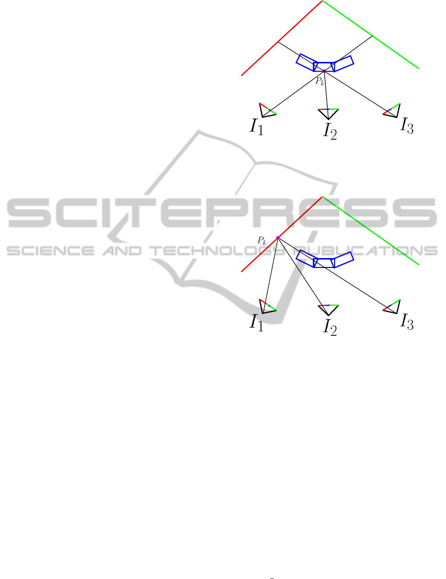
2.5.3 Photo-consistency Criterion Computation
It is very important to understand that, since there are
moving objects in the camera and in the 3D point
cloud, the photo-consistency will be wrong for any
point, static or not, because moving objects are in
camera images. So a static point will have a bad
photo-consistency error in images where a moving
object stands in front of it. On the contrary, a 3D
point on a moving object is photo-consistent in all the
images where it was not moving. This problem is re-
ally hard to solve because image data are biased by
moving object, but there is a solution. A point on a
static object is photo-consistent (figure 5) anywhere
except on images with a moving object, but a point
on a moving object is photo-consistent only in images
where this moving object was there (figure 4). So the
two types of object can be distinguished by a principal
mode extraction as we seen in figure 5.
To this end, a kernel density estimator will be
used as a Gaussian mixture model to find the prin-
cipal mode in the set of the color descriptor vector
C . If C
k
∈ C and C
l
∈ C are to color vector descrip-
tor coming respectively from I
k
and I
l
. A SSD score
noted D
k,l
estimates the similarity between them by
using L
2
norm of the difference of colors. The D
i, j
Figure 4: A point taken on a moving object is only photo-
consistent in the image where it is visible (I
2
). In the other
images it is never consistent. Here it has three different col-
ors: blue, green and red.
Figure 5: A static point can be partially photo-consistent
because its colors are: red, red and blue. But there is a
consistent principal mode: red.
are computed for all the (i, j) pairs and regrouped in
a distance matrix.
D
c
=


D
1,1
... D
1,n
... ... ...
D
n,1
... D
n,n


(1)
To extract a sample consensus from this matrix,
a Gaussian kernel with a standard deviation of σ is
applied to each term of the distance matrix, the rows
are summed and the column cmax with the highest
score is selected. This column represent the descrip-
tor nearest to the principal mode of the estimated
density of probability for the descriptors distribution.
The value of this mode (the maximal value of the
sum of the column) is our photo-consistency crite-
rion: J
j
=
1
n
n
∑
i=1
D
i,cmax
associated to the 3D point P
j
.
In many photo-consistency algorithms, the criterion is
not robust to outliers and do not tolerate any problem.
With this solution, the criterion is robust to outliers,
ICPRAM2014-InternationalConferenceonPatternRecognitionApplicationsandMethods
812

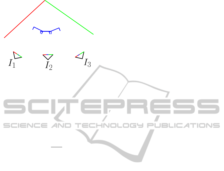
Figure 6: The eroded scene after one iteration. The 3D
points on the blue car are disappearing and let the back-
ground appear which is photo-consistent.
deal with occlusion and is totally symmetric from the
point of view of images. No image is used as refer-
ence, no preferences or a priori are done on the im-
age set or on the surface.The parameter σ is chosen as
6σ
ph
where σ
ph
is the standard deviation of the sensor
noise (ie. photogrammetric noise on pixels value).
This phase is computationally intensive with mil-
lions of 3D points and hundred of images because for
a point seen in n images,
n(n−1)
2
descriptor distance
are computed. So we choose the SSD as distance be-
cause it is very fast. SSD is not robust to illumina-
tion change but in our case, the images are taken in a
short time so the illumination is similar. As example,
a scene with 20 images, 1 millions 3D points seen in
an average of 7 images per points, the total computa-
tional time including clipping and z-buffer is 10s on
a Quad-Core 3.2Ghz where 80% of the time is con-
sumed in photo-consistency score estimation.
2.6 Scene Erosion
The photo-consistency score J
j
is analyzed to esti-
mate if a point needs to be removed or not. For this
step, a simple threshold S
e
is used : all the points in-
ferior to S
e
are deleted from the point database and
from the octree, otherwise nothing is done (figure 6).
By the way, the 3D scene is eroded and the process
restarts at the step (2.3) until all the scene points are
photo-consistent. At the end of the IPCC algorithm,
the photo-consistent scene is returned and the deleted
points are stored in a list. Static and moving objects
are classified in the 3D world but not in the images.
The classification in the images is left to the next sec-
tion.
2.7 Image Inpainting
After the end of the Iterative Photo Consistency
Check algorithm, the point cloud P contain only static
and photo-consistent point. The main idea to detect
moving object in images is to compute a last time
all the step of the method and stop to the photo-
consistency criterion step (2.5). This time, we don’t
want to estimate if the 3D point is moving or not, but
we want to estimate in which images it is not photo-
consistent and inpaint this area. By the way, image
inpainting is computed in three step : first a photo-
consistency score is computed over all the pixel of
the image I
k
defining a probability field M
k
. Secondly,
this probability is thresholded to obtain a binary map
B
k
. Then all the area of B
k
with value 0 are inpainted
by 3D surface regression and pixel re-projection in
the image I
cmax
. An application on the example can
be seen in figure 7.
2.7.1 Probability Field Estimation
In fact, the solution is already in the distance ma-
trix D
i, j
, because after the application of the Gaussian
kernel, the column with the largest sum define the
best photo-consistent color descriptor but the proba-
bility than the best photo-consistent color descriptor is
photo-consistent in the image I
k
is given by the value
of F
k
= D
k,cmax
. Where k is the image index and cmax
is the column index of the principal mode.
So for each point P
j
∈ P seen in I
k
, a photo-
consistency score is given for this image. But the
image is a pixel matrix and we only compute photo-
consistency on the set of sparse 3D points which are
visible in I
k
. So, it is necessary to project the 3D point
cloud in I
k
and interpolate the probability of being a
photo-consistent object on each pixel (i, j) to obtain a
dense probability map M
k
. To this end, sparse data are
interpolated with a robust method : the median of the
nearest neighbor value. This solution consist to find
the 3D points projected in I
k
and near from coordinate
(i, j) then collect them probability value and take the
median as the value of pixel (i, j) of M
k
. An example
of probability field M
k
can be seen in the experimental
section 3.
2.7.2 Thresholding and Inpainting
The probability map M
k
is then thresholded by the
same value as the 3D point in the scene erosion : S
e
.
We obtain a binary map B
k
where all value equal to
0 need to be inpainted. For each pixel p
i, j
∈ B
k
with
value 0, we want to find a color to replace the old
one. This new color can be found in another image
where the scene is photo-consistent, but it is a local
TowardMovingObjectsDetectionin3D-LidarandCameraData
813

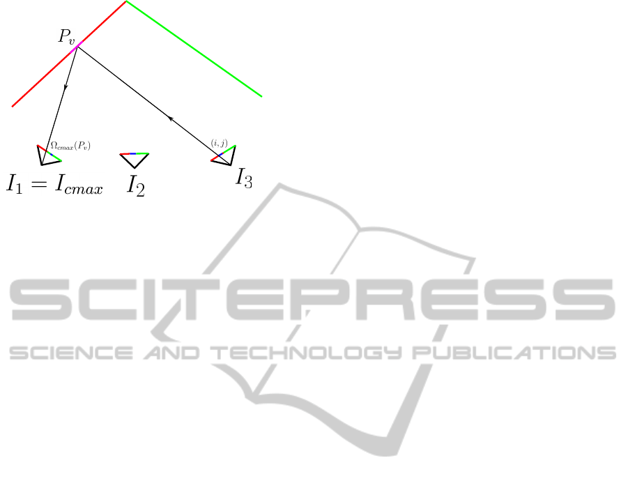
Figure 7: Principle of Image inpainting. The color C
k1
from
image I
1
and C
k2
from I
2
are averaged to obtain the color
C
k
of point P
k
. This one is projected in the non consistent
image I
3
and the images pixels are fixed.
parameter because a part of the inpaint can be better
in image I
q
and another part can be good in I
m
. To
determine which image will be used to inpaint a pixel
(i, j) of image I
k
, we chose to look for the visible 3D
point projected in I
k
and nearest to coordinate (i, j).
Let P
s
this point, so the locally best photo-consistent
image is I
cmax
where cmax is the index of the column
corresponding to the principal mode for the point P
s
.
Once the image I
cmax
is find for the pixel p
i, j
, we
need to determine which pixel of I
cmax
will be use to
fill the pixel (i, j) of I
k
. The only solution is to back
project a ray from (i, j) in image I
k
on the 3D sur-
face to obtain a virtual 3D point P
v
, and project it
in the image I
cmax
using Ω
cmax
to find it color (via
a bi-cubic interpolation). This method can be done
because the erosion delete all moving object and let a
photo-consistent scene, the 3D surface become differ-
entiable and we are able to compute a 3D surface esti-
mation. To this end, we use the 3D points projected in
I
k
and nearest from coordinate (i, j) as in 2.7.1 and we
compute a moving least square (Cheng et al., 2008)
regression of the depth value of this point set using a
polynomial of degree two. So an interpolated depth is
computed in (i, j), the inverse projection function give
the needed virtual 3D point P
v
then the pixel color is
locally fixed by the color of Ω
cmax
(P
v
) in image I
cmax
.
In all our experiment, nearest neighbour interpolation
and regression is done with the 15 nearest data.
3 APPLICATION TO SEQUENCE
3.1 Methodology
In order to test our algorithm and prove the possibil-
ity of detecting moving objects in both camera and
range-data with non synchronous sensors, our method
has been applied to a synthetic dataset. We consider
a outdoor scene, in front of a shop where a pedestrian
come from the right and go to the left in the cam-
era. This represents the type of scenes that motivated
our approach, in the context of robotic applications,
where a vehicle would take pictures of its environ-
ment. This sequence was made by a realistic sen-
sor simulator (4D-Virtualiz (Delmas, 2011; Malartre,
2011)) which generates data from a color camera and
a Velodyne HDL-64E. Both sensors are positioned on
a mobile vehicle going forward. The Velodyne is a
3D panoramic lidar with 64 lasers, an angular resolu-
tion of 0.09 degrees and a precise depth information
(σ = 0.05m). This sensor acquires a massive point
cloud with 1.3 millions point by second all around
it. The color camera has a resolution of 1024 × 768,
a frame rate of 15 f ps, and positioned to look at the
left side of the vehicle. For all theses data, the sen-
sors pose ground truth is used to realign the range
data and the camera poses in the common reference
system. This test sequence contain 4.10
6
3D points
acquired by the Velodyne and 52 pictures. A example
image can be seen in figure 8. For this experiment, we
choose a probability threshold of S
e
= 0.4.
After the execution of our method, points are clas-
sified in static or moving object. In order to analyze
our results, we define five statistics indicator :
1. Pt : The number of 3D points detected on static
objects which is really on a static object (true pos-
itive)
2. Nt : The number of 3D points detected on moving
objects which is really on a moving object (true
negative)
3. P f : The number of 3D points detected on static
objects which is not really on a statics object (false
positive)
4. N f : The number of 3D points detected on mov-
ing objects which is not really on a moving object
(false negative)
3.2 Results, Analysis and Discussion
The Figure 8 show the original image from the exper-
imental sequence. IPCC algorithm is then applied to
this image set and to the corresponding point cloud
to delete all non-photo-consistent 3D points. The Ta-
ble 1 presents informations about the dataset for each
iteration of the IPCC algorithm. We can see that
only 263.10
3
points are selected by the clipping and
the Z-buffers. This points are seen in an average of
6 images, that is sufficient to find a principal mode
by using our photo-consistent criterion. By the way,
ICPRAM2014-InternationalConferenceonPatternRecognitionApplicationsandMethods
814

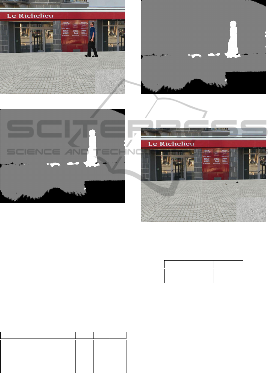
Figure 8: Example image of the simulated sequence.
Figure 9: An image corresponding to the interpolated prob-
ability field M
k
, in image I
k
. Gray is moving, White is static
and Black is unknown because there is not enough neigh-
bors.
the first iteration remove 8314 points, the second 467
and the scene is totally photo-consistent at the 6-th
iteration. The Table 2 present statistical information
about the point cloud classification. Our filter is very
strict with static objects because the positive predic-
tive value is equal to 99.40% and has a good negative
predictive value of 96.80%. So our filter is very strict
but better to remove objects than to extract moving
objects, it is due to an higher value of the negative
false.
Table 1: Algorithm statistics over iterations.
Iterations 1 2 3
Occurrence list size (10
3
) : 217 262 263
Average occurrence per points 6.4 6.99 7.66
Number of removed points 8314 467 78
Computation time (s) 12 12 11
Image inpainting time (s) 10
Figure 10: An image corresponding to the thresholded
probability field B
k
. Gray is static, White zone need to be
inpainted and Black is unknown because there is not enough
neighbors.
Figure 11: A inpainted image using MLS (Moving
Least Square) interpolation of surface and pixel color re-
projection.
Table 2: Point cloud classification statistics.
10
3
Positive Negative
True Pt = 264 Nt = 1.6
False P f = 0.1 N f = 7.1
Image 9 show an example of interpolated proba-
bility field and Figure 10 is the thresholded value of
M
k
. We can see in this qualitative result of our algo-
rithm that the detection of the person is precise but we
can see that his feet where not detected as moving ob-
ject. The reason of this miss-detection is that the color
of the floor is gray from any point of view so the 3D
points near the floor (the feet of the pedestrian) are
considered photo-consistent. Figure 11 show the im-
age after inpainting pixel color value with the value
of another image via the interpolated surface using
MLS. Classification performance and image inpaint-
TowardMovingObjectsDetectionin3D-LidarandCameraData
815

ing are clearly improved in comparison to the original
article (Clement Deymier, 2013a).
The IPCC algorithm complexity is evaluated to
O(n
3
m × log(m)) where n is the number of camera
and m is the number of points in the scene. But if
we consider that a 3D points is only seen in a small
number of camera : τ (It is often the case when the
mobile vehicle is acquiring) then the algorithm com-
plexity become : O(τ
2
nm × log(m)). The method be-
come scalable to very long sequence with millions of
points and hundred of images. The number of iter-
ation necessary to remove all 3D points depend on
volume and trajectory of the moving objects but in
our experiments, after six iteration the scene is always
close to be totally photo-consistent.
4 CONCLUSIONS AND FUTURE
WORK
The objective of this article was to improve the photo-
consistency estimation and to demonstrate the effi-
cacy of the IPCC algorithm. It present an original
method to detect moving object both in camera and
in range data. The core of the problem, the non syn-
chronous acquisition of the data is solved by using a
time-independent photo-consistency criterion applied
on the entire sequence. This criterion use a princi-
pal mode extraction in color descriptor vector space
to find the statics points in the sequence and the non
photo-consistent point are classified as moving and
deleted from the scene. The iterative aspect of this
algorithm allow to detect all the 3D points on the
moving object and not only it surface. Moreover, this
method is very flexible because more than one range
finder or camera can be used since the cloud is dense
enough and the camera are in color.
REFERENCES
Cheng, Z.-Q., Wang, Y.-Z., Li, B., Xu, K., Dang, G., and
Jin, S.-Y. (2008). A survey of methods for mov-
ing least squares surfaces. In Proceedings of the
Fifth Eurographics / IEEE VGTC conference on Point-
Based Graphics, SPBG’08, pages 9–23, Aire-la-Ville,
Switzerland, Switzerland. Eurographics Association.
Clement Deymier, T. C. (2013a). Ipcc algorithm: Moving
object detection in 3d-lidar and camera data. In IEEE
Intelligent Vehicles Symposium.
Clement Deymier, Damien Vivet, T. C. (2013b). Non-
parametric occupancy map using millions of range
data. In IEEE Intelligent Vehicles Symposium.
Delmas, P. (2011). Gnration active des dplacements d’un
vhicule agricole dans son environnement. PhD the-
sis, Ecole Doctorale Science Pour l’Ing
´
enieur de Cler-
mont Ferrand.
Fujimoto, K., Kimura, N., and Moriya, T. (2012). Method
for fast detecting the intersection of a plane and a cube
in an octree structure to find point sets within a convex
region. In Society of Photo-Optical Instrumentation
Engineers (SPIE) Conference Series, volume 8301 of
Society of Photo-Optical Instrumentation Engineers
(SPIE) Conference Series.
Himmelsbach, M. (2008). Lidar-based 3d object percep-
tion. Proceedings of 1st International Workshop on
Cognition for Technical Systems.
Jung, B. and Sukhatme, G. S. (2004). Detecting moving
objects using a single camera on a mobile robot in an
outdoor environment. In in International Conference
on Intelligent Autonomous Systems, pages 980–987.
Malartre, F. (2011). Perception intelligente pour la nav-
igation rapide de robots mobiles en environnement
naturel. PhD thesis, Ecole Doctorale Science Pour
l’Ing
´
enieur de Clermont Ferrand.
Royer, E., Lhuillier, M., Dhome, M., and Lavest, J. (2007).
Monocular vision for mobile robot localization and
autonomous navigation. International Journal of
Computer Vision, 74:237–260. 10.1007/s11263-006-
0023-y.
Rusinkiewicz, S. and Levoy, M. (2001). Efficient variants
of the icp algorithm. In International Conference on
3-D Digital Imaging and Modeling.
Slabaugh, G. G., Culbertson, W. B., Malzbender, T.,
Stevens, M. R., and Schafer, R. W. (2003). Methods
for volumetric reconstruction of visual scenes. Inter-
national Journal of Computer Vision, 57:179–199.
Wurm, K. M., Hornung, A., Bennewitz, M., Stachniss, C.,
and Burgard, W. (2010). OctoMap: A probabilis-
tic, flexible, and compact 3D map representation for
robotic systems. In Proc. of the ICRA 2010 Workshop
on Best Practice in 3D Perception and Modeling for
Mobile Manipulation, Anchorage, AK, USA.
Yilmaz, A., Li, X., and Shah, M. (2004). Contour based
object tracking with occlusion handling in video ac-
quired using mobile cameras. IEEE Transactions on
Pattern Analysis and Machine Intelligence, 26:1531–
1536.
Zeng, G., Paris, S., Quan, L., and Sillion, F. (2005). Pro-
gressive surface reconstruction from images using a
local prior. In In ICCV, pages 1230–1237.
Zografos, V., Nordberg, K., and Ellis, L. (2010). Sparse
motion segmentation using multiple six-point consis-
tencies. CoRR, abs/1012.2138.
ICPRAM2014-InternationalConferenceonPatternRecognitionApplicationsandMethods
816