
Diagnostics of Coronary Stenoses
Analysis of Arterial Blood Pressure Signals and Mathematical Modeling
Natalya Kizilova
Kharkov National University, Svobody sq., 4, Kharkov, Ukraine
Keywords: Arterial Blood Pressure, Pulse Wave, Coronary Arteries, Stenosis, Mathematical Modelling, Pressure, Flow
Signal Processing.
Abstract: Severity of the coronary stenoses and necessity of the percutaneous coronary intervention is usually
estimated basing on analysis of the pressure and flow signals measured in vivo by a pressure gauge at
certain distances before and after the stenosis. In the paper the differences in the pressure gradients at
different stenosis severity are shown and discussed. A method of decomposition of the measured biosignals
into the mean and oscillatory components is proposed. A mathematical model of the steady and pulsatile
flow through the viscoelastic blood vessel in the presence of the rigid guiding wire is developed for
biomechanical interpretation of the measured coronary blood pressure and flow signals. A novel approach
for estimation the stenotic severity basing on the measured and computed data is proposed.
1 INTRODUCTION
Coronary artery disease, which is also known as
atherosclerotic or ischemic heart disease, has
become one of the most severe diseases causing a
large number of deaths each year over the world.
The partial occlusion of the stenosed artery and
abnormal blood flow through it to the heart cells
lead to insufficient oxygen delivery, especially when
the possibilities of the perfusion regulation by the
resistive coronary vessels are spent (Vlodaver at al,
2012). The causes to the formation of atherosclerotic
lesions and arterial stenosis are still unknown but it
is well established that the fluid dynamics,
particularly the wall shear stress (WSS) and local
pressure oscillations play an important role in the
genesis of the disease (Layek et al, 2009).
In the absence of stenosis, the driving pressure
gradient is constant over the coronary vessels. With
progressing of the stenosis severity, the pressure
gradient required to impel the blood through the
narrowed path increases that results in a higher
blood pressure at the inlet of the stenosed artery. The
heart must work harder to increase the produced
pressure, and when the blood supply to the working
heart is insufficient the angina and even heart attack
may occur. In-time diagnostics of the stenosed
coronary arteries is crucial for timely therapy or/and
surgery of the coronary lesions.
Coronary angiography (AG), intravascular
ultrasound (IVUS) and coronary computed
tomography angiography (CCTA) are commonly
used for estimation of the stenosis severity by
computations of the minimal lumen area (MLA) that
is determined as the ratio of the minimal A
min
to
normal A
0
lumen areas: MLA= A
min
/A
0
(%). The
results of the AG, CCTA and IVUS-based MLA
computations correspond well to each other (Caussin
et al, 2006), but not in the case of the calcified wall
(Li Y. and Zhanga, 2012). MLA gives geometric
approximation of the stenosis and in many cases the
stenoses with MLA<50% remain insignificant and
do not need stenting or bypass surgery, because
sufficient perfusion is provided by autoregulation of
the resistive vessels and collateral blood supply.
The functional severity of the stenosis can be
estimated by the fractional flow reserve (FFR)
defined as the ratio of the mean distal P
d
and
proximal (anterior) P
a
coronary pressures measured
via the pressure wire at certain distances before and
after the stenosis during maximal hyperemia
produced by intravenous adenosine administration
that leads to relaxation of the myocardial vessels.
The normal FFR=0.94–1.0, whereas the FFR<0.75
highly correlates with insufficient perfusion and
myocardial ischemia. The patients from the grey
zone 0.75<FFR<0.8 may have had a risk of ischemia
(Silber et al, 2005; Pijls, 2003). FFR reveals the
76
Kizilova N..
Diagnostics of Coronary Stenoses - Analysis of Arterial Blood Pressure Signals and Mathematical Modeling.
DOI: 10.5220/0004929500760083
In Proceedings of the International Conference on Bio-inspired Systems and Signal Processing (BIOSIGNALS-2014), pages 76-83
ISBN: 978-989-758-011-6
Copyright
c
2014 SCITEPRESS (Science and Technology Publications, Lda.)

dangerous ischemia-producing lesions (Tonino,
2010), and it is recognized as gold standard for
assessing the hemodynamic significance of coronary
stenoses (Finn et al, 2012). The similar approach
based on the flow velocities at rest and the
hyperaemic state has also been developed.
Computational fluid dynamics (CFD) is widely
used in advanced studies on the blood flows in rigid
and compliant boundaries. The corresponding finite
element and finite volume models and the
computational schema have been used for the blood
flow modeling in the vessels of different size up to
the cellular level (Hinds et al, 2001). CFD study of
the flow past symmetric and asymmetric stenoses in
the straight, curved, helical and bifurcating tubes
allow computations of the FFR values for every
single stenosis as well as for the tandem,
overlapping and bifurcational lesions. CFD approach
allows virtual planning and estimation the outcomes
of the surgery (stents, grafts, bypass) (Xiong, 2012),
and the computed tomography (CT)-based virtual
FFR estimation is a challenge that is widely
discussed in recent publications (Taylor et al, 2013;
Qi et al, 2013; Rajani et al, 2013). In the present
paper some novel aspects of the FFR assessment and
analysis of the measured pressure signals are
proposed and discussed basing on the measurement
data and the mathematical model of the blood flow
in different rigid and compliant boundaries.
2 BLOOD PRESSURE SIGNALS
2.1 The Measurement Procedure
CFD computations and virtual FFR estimations are
based on the 3D models of the viscous
incompressible blood flow in the rigid patient-
specific geometry of the larger epicardial coronary
vessels recognized in AG and CCTA images, while
the invasive FFR calculations are based on the in
vivo measurements of the blood pressures before and
after the stenosis at the presence of the guiding
catheter and wire.
At local anesthesia, a guide catheter (Figure 1) is
inserted into the orifice of the coronary artery
through the femoral or radial artery. The pressure
and flow signals in the coronary arteries can be
measured by the pressure and Doppler guide wire
(2). The diameters of the catheters can be chosen
between d=1.5–2.3 mm, while the manufactured
guidewires have the diameters d=0.35–0.89 mm.
According to the measurement data (Dodge,
1992), the main coronary arteries of adult humans
Figure 1: Schematic representation of the intravascular
coronary examination: the guide catheter (1) in the
coronary artery (2) and the guidewire with pressure and
flow gauges (3) in the coronary stenosis (4).
have the following diameters: d=4.5±0.6 mm for the
left main artery; d=3.7±0.4 mm and d=1.9±0.4 mm
for the proximal and distal parts of the left anterior
descending artery; d=3.4±0.5 mm for the left
circumflex artery; d=3.9±0.6 mm and d=2.8±0.5 mm
for the right coronary artery. The comparison of the
diameters shows that both the catheter and wire can
produce disturbances in the natural coronary blood
flow and wave propagation.
In this study 45 data samples recorded in the
epicardial coronary arteries of 32 patients with
different stenosis severity diagnosed by the pressure
gauge administrated via the guiding catheter have
been analyzed. An example of the recorded rata
digitized from the CathLab software is presented in
Figure 2. The red and green time-varying curves
correspond to the pressure signals P
a
(t) and P
d
(t)
accordingly, while the relatively smooth red and
green lines correspond to their mean values. The
measurements have been carried out during the
adenosine administration which dynamics can be
followed by the shift between the both oscillating
and mean value curves. The FFR value indicated
with yellow color has been computed automatically
Figure 2: An example of the pressure signals recorded in
the coronary artery by the pressure gauge and analyzed by
the CathLab software.
DiagnosticsofCoronaryStenoses-AnalysisofArterialBloodPressureSignalsandMathematicalModeling
77
by the CathLab software.
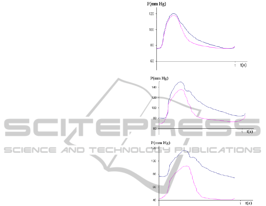
2.2 Smooth and Oscillatory Signals
Depending on the presence and severity of the
stenosis, the pressure gradients in the signals
measured before P
a
(t) and behind P
d
(t) the stenosis
have significant differences. As the stenosis severity
is progressing, the pressure behind the lesion drops
first in diastole, while the pressure decrease after the
peak systole is the same as in the pressure signal
P
a
(t) (Fig.3a). Then the pressure drop in diastole
becomes more significant (Fig.3b) and the
differences in the pressure gradients appear also in
the systole (Fig.3c).
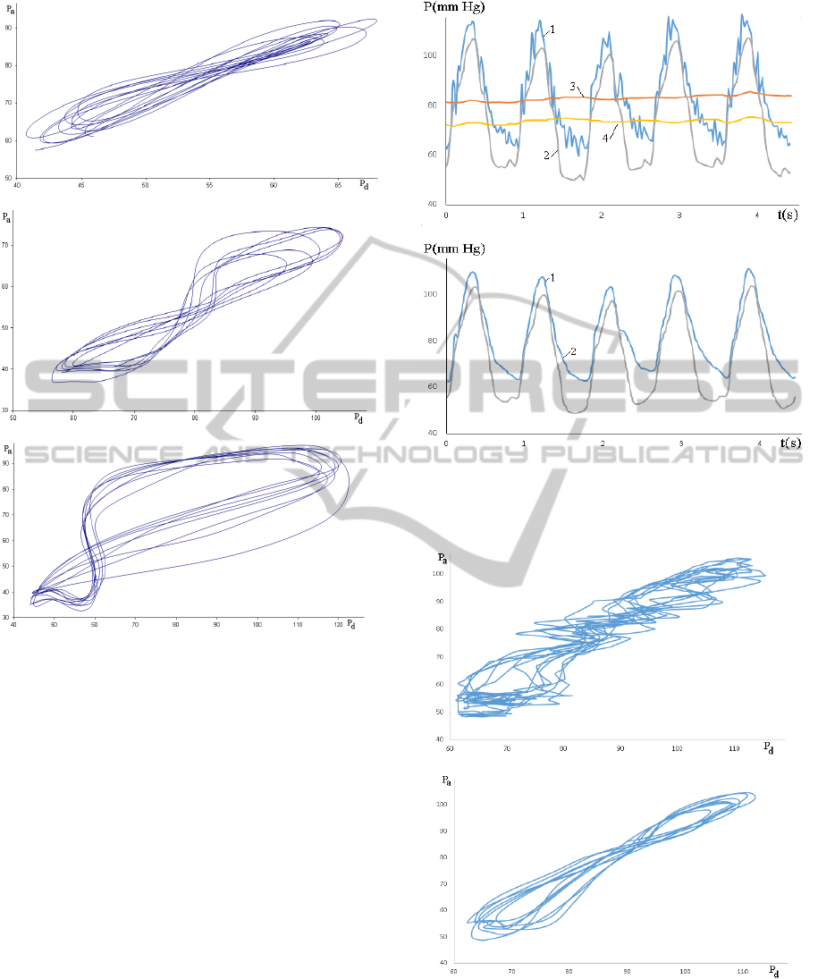
The contour analysis of the
P
a
(t) and P
d
(t) signals
characterises their relative differences in slopes and
values, while some novel information important for
diagnostics can be driven from the P
a
(P
d
), pressure-
flow P(U), and phase curves P
/
(P) and U
/
(U)
computed from the measured signals where the
stroke sign denotes the time derivative (Kizilova,
2013). For instance, the P
a
(P
d
) curves computed
from the P
a
(t) and P
d
(t) signals by elimination of
time are presented by loops (Fig.4) slightly varying
according to the heart rate, blood pressure and flow
variability (Barclay et al, 2000; Trzeciakowski and
Chilian, 2008). In spite of the heart rate and blood
perfusion variability, the characteristic shape of the
loop is preserved from beat to beat. When the
myocardial perfusion is normal, the P
a
(P
d
) loop is
elongated and tends to the straight line (Fig.4a).
When the stenotic flow is critical in the term of
the FFR values, the loop is shaped as digit ‘8’ and
the self-intersection point is located in the middle of
the loop (Fig.4b). When the perfusion is insufficient,
the FFR value is low and the urgent surgery is
necessary, the P
a
(P
d
) becomes ‘thicker’ and is
looking as asymmetric ‘8’ because of the
asymmetric location of the self-interaction point
(Fig.4c). Similar changes in the shapes of the
dependencies (P
a
–P
d
) on P
d
and (P
a
–P
d
) on P
a
with
progressing stenotic severity (functional, not
geometrical!) have been observed in this study.
Representation of the measured blood pressure
signals as cycles allows computation of different
integral parameters like the area located inside the
loop and its two subparts produced by the
intersection point, variability of its location and
slope.
The measured blood pressure signals P
a
(t)
sometimes exhibit oscillating behaviour (Fig.5a),
while in many cases they remain relatively smooth
(Fig.3). Note that the P
d
(t) curves do not
a
b
c
Figure 3: Blood pressure signals P
a
(t) (upper lines) and
P
d
(t) (lower lines) measured in the epicardial coronary
arteries with progressing stenosis severity (a,b,c).
demonstrate such oscillating behaviour, because the
stenosis serves as the wave absorber producing
reflected waves that propagate in the upstream
direction and appear in the P
a
(t) signal. Similar
regularity has been found in (Canic, 2006).
Numerical simulations on the 1D model exhibit
high-frequency, short wave-length reflected waves
superimposed over the main wave front, and the
computed high frequency oscillations were not a
consequence of the numerical solver. Applying the
3–5 point smoothing filters or eliminating the high
harmonics from the Fourier expansion, the P
a
(t)
signals may be transformed in the smooth curves,
but the computed FFR values will be always lower
for the initial P
a
(t) (oscillatory) signals than for the
smoother ones, because the smoothing procedure
cuts the high oscillations and decreases the mean
values of the signals. In that way the FFR computed
on the oscillating curves can overestimate the
BIOSIGNALS2014-InternationalConferenceonBio-inspiredSystemsandSignalProcessing
78
a
b
c
Figure 4: P
a
(P
d
) loops for the stenotic flows at FFR=0.86
(a); FFR=0.7 (b); FR=0.53 (c).
stenosis severity. The smoothing leads to elimination
of information that can be complementary to the
FFR value and useful for more detailed diagnostics
of the stenosis rigidity or presence of the atheroma,
thrombus and fibrous cap. The P
a
(P
d
) loops
computed from the oscillating (Figure 6a) and
smoothed (Figure 6b) pressure signals (see Figure 5a
and 5b correspondingly) demonstrate the intensity of
the high-frequency oscillations produced by
additional wave reflection. The smoothed curves
(Figure 5b) still can be classified and explained in
correspondence to the examples presented in Figure
4, while the oscillating ones (Figure 5a) needs
elaboration of new indexes and their biomechanical
interpretation.
The pulsatile component of the measured
pressure signals is not taken into account in the FFR
computations, so decomposition of the signal P(t)
into the mean <P(t)> and oscillatory P/(t) terms and
a
b
Figure 5: In vivo measured pressure curves before (a) and
after (b) the smoothing procedure – P
a
(t) (1), P
d
(t) (2), <
P
a
(t)> (3), <P
d
(t)> (4).
a
b
Figure 6: P
a
(P
d
) loops for the oscillatory (a) and smoothed
(b) pressure signals presented in Figures 5 a and 5b
accordingly.
examination of the oscillatory component may be
interested for the diagnostic purposes, as well as for
DiagnosticsofCoronaryStenoses-AnalysisofArterialBloodPressureSignalsandMathematicalModeling
79

deeper understanding the blood flow and pressure
wave propagation through the stenosis. Fir instance,
the FFR values could be computed separately for the
mean and oscillatory components as
FFR=
<P
d
(t)>/< P
a
(t)> and FFR
osc
= P/
d
(t)/ P/
a
(t).
A comparative analysis of the FFR, FFR
osc
and
MLA values on a large representative group of the
measurements in the stenosed arteries will be done
in the next studies.
3 MATHEMATICAL MODEL
3.1 Steady Blood Flow between the
Rigid Boundaries
The simplest model of the blood flow in the stenosed
artery in the presence of the guide catheter (Fig.1) is
the steady viscous flow between the rigid coaxial
cylinders. According to the well-know solution of
the problem the axial flow is
22
22
21
2
21 2
RR
Pr
V(r) R r ln
4L ln(R/R) R
(1)
where
2
R is the radius of the artery,
1
R is the
radius of the wire/catheter,
is the blood viscosity,
L
is the distance between locations of the proximal
and distal measurement sites,
P
is the measured
pressure drop.
The virtual FFR in the straight part of the blood
vessel is computed on the CFD model that in the
limit of the rigid wall and the steady inflow tends to
the Poiseuille solution
22
P2
P
V(r) R r
4L
(2)
From (1) and (2) the error in the FFR values
computed basing on the measurement signals and
CFD computations can be estimated.
3.2 Pulsatile Blood Flow in Compliant
Vessels
Heart contraction produces oscillations of the
pressure and flow that propagate along the vessels,
and the speed of the pulse waves vary from c=5–8
m/s in large elastic arteries to c=10–12 m/s in small
resistive blood vessels. In elderly individuals and in
the case of atherosclerosis, hypertension and some
other cardiovascular disorders the pulse wave
velocity increases up to c=25 m/s (Nichols et al,
2011). The wave propagation and reflection at the
arterial branching, atherosclerotic plaques, lesions
and other non-uniformities produce complex
superposition of the propagated and reflected waves.
Spectral and wave-intensity analysis of the
registered signals can reveal novel features of
hemodynamics of stenosis and diagnostic indexes.
In this paper the axisymmetric wave propagation
between the coaxial cylinders is proposed as the
model of the pulsatile blood flow and pressure wave
propagation in the compliant artery when the
guiding catheter is inserted (Fig.1).
Fluid flow is governed by incompressible
Navier-Stokes equations
2
v0,
v
(v )v p v,
t
(3)
the mass and momentum conservation equations for
the incompressible vessel wall
2
ws
2
u0,
u
ˆ
p
,
t
(4)
where
v
is the flow velocity,
u
is the wall
displacement,
and
w
are the mass densities for
the blood and wall,
is the fluid viscosity, p and
s
p
are the hydrostatic pressures in the fluid and
solid,
ˆ
is the stress tensor for the vessel wall.
The viscoelastic Kelvin-Voight body has been
used as rheological model for the layers:
iw i ikkw k
A
tt
(5)
where
ik
A
is the matrix of elasticity coefficients,
w
is the wall viscosity,
w
is the stress relaxation
time,
T
11 22 33 23 13 12
,,,,,
is the stress
vector,
is similar strain vector,
ik i k k i
(u u)/2
, T is transposition sign.
The boundary conditions include the no-slip flow
condition at the inner rigid surface; continuity
conditions for the fluid and solid velocities and the
stress components at the fluid-wall interface:
1
rR:v0
(6)
2nn
du
rR :v ,
dt
(7)
At the outer surface of the blood vessel the no
displacement or no stress boundary conditions can
be taken in the form
BIOSIGNALS2014-InternationalConferenceonBio-inspiredSystemsandSignalProcessing
80

2n
rR h: 0oru0
(8)
where h is the thickness of the arterial wall, n and τ
denotes the normal and tangential components.
At the ends of the tube the fastening conditions
for the tube
z0;L:u0,
(9)
the input wave at the inlet and the wave reflection
condition at the outlet of the tube
0
z 0 : p(t,0) p (t),
(10)
0
z L : p(t, L) p (t),
(11)
where
is the complex reflection coefficient equal
to the ratio of the amplitudes of the reflected and
propagates waves (Nichols et al, 2011),
Re( ) [0,1]
and
Im( )
corresponds to resistivity
and capacity of the downstream vasculature
(Lighthill, 2001) are considered.
The solutions of the problem (3) and problem
(4)–(5) which are coupled via the boundary
conditions (8)–(11) have been found as a
superposition of the steady solution and small
axisymmetric disturbance in the form of the normal
mode:
** stikz
** stikz
v, p v , p v ,p e
u,p u ,p u ,p e
where
v
,
u
,
p
,
s
p
are the amplitudes of the
corresponding disturbances,
ri
kk ik
,
ri
ss is
,
i
s
is the wave frequency,
r
k
is the
wave number,
r
s
and
i
k
are spatial and temporal
amplification rates, z is the axial coordinate. The
steady part
**
,
vp
is identified with Poiseuille
flow (1) between the rigid surfaces.
The amplitudes
v
,
u
,
p
,
s
p
can be
obtained from (3)–(4) as Fourier expansions
jj
n
i( t x)
1j 0 j
j0
p
CJ(i r)e ,
jj
n
rj2j1j3j1j
j0
i( t x)
10 j 0 j 11j 0 j
Vi(CJ(ir)CJ(ir)
CK(ir)CK(r))e ,
jj
n
x2jj1j3jj1j
j0
i( t x)
10 j 0 j 11j 0 j
V i(C J(i r) C J(i r)
C K (i r) C K ( r))e ,
(12)
jj
n
i( t x)
s8j0j9j0j
j0
p
(CJ(ir)CY(ir))e ,
jj
n
r j 4j1j 5j1j
j0
6j1j 7j1j
i( t x)
12 j 1 j 13 j 1 j
Ui(CJ(r)CY(r)
C J (i r) C Y (i r)
CK(ir)CK(r))e ,
jj
n
x4jj0j5jj0j
j0
6j j 0 j 7j j 0 j
i( t x)
12 j 0 j 13 j 0 j
U(CJ(r)CY(r)
Ci J(i r) Ci Y(i r)
CK(ir)CK(r))e .
where
22
jj j
i
,
22 2
jjwwj
,
jjj
/c
,
j
c
is the speed of the j-th harmonics,
kj
C
are unknown constants,
0,1
J
,
0,1
Y
are Bessel and
0,1
K
are modified Bessel functions of the 1
st
and 2
nd
kind.
The difference of the obtained solution (12) and
the well-known Womersley solution at different
boundary conditions (Cox, 1968; Milnor, 1989) is
the modified Bessel functions
0,1
K
in the
expressions of the fluid velosities and wall
displacements which become infinite at r=0 and,
therefore, are absent in the Womersley solution for
the hollow tube (at
1
R0
). The constants
kj
C
can
be obtained by substitution of (12) into the boundary
conditions (6)–(11). The resulting expressions are
not present here because of their complexity.
4 RESULTS AND DISCUSSIONS
The pressure and flow distributions in the pulsatile
flow between the coaxial rigid (guiding
catheter/wire) and compliant viscoelastic surfaces
have been computed on (9) using the following
physiological parameters: ρ=1050 kg/m
3
, ρ
s
=1000–
1300 kg/m
3
, μ=3.5·10
-3
Pa·s, μ
s
=1 Pa·s, τ
s
=0.01–
0.1 s, R
1
=0.18–1.25 mm, R
2
=0.75–2.5 mm,
Re( )
0; 0.5;0.9
,
Im( ) 1 i
. The computed
p
(t,r,x)
and
v(t, r, x)
distributions have been
averaged over the cross-sectional area between the
two surfaces and then compared to the solutions of
the same problem formulation (3)–(11) at R
1
=0
(Lighthill, 2001). The aim of the study was to check
whether the pressure signals measured for the
pulsatile blood flow between two surfaces and in
some cases in quite a narrow gap between them
((R
2
–R
1
)/R
2
~0.5–0.75) are consistent with the CFD
DiagnosticsofCoronaryStenoses-AnalysisofArterialBloodPressureSignalsandMathematicalModeling
81
computations for the flows in rigid tubes without the
axial obstacles (Taylor et al, 2013; Qi et al, 2013;
Rajani et al, 2013). The input pressure waveforms
0
p
(t) and the wave reflection coefficients
have
been taken in the same form for both geometries.
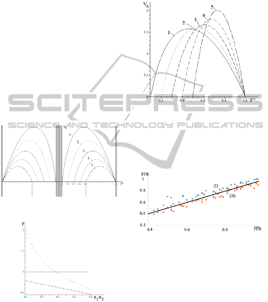
The non-dimensional axial flow profiles
V
x
(r°)
computed at the same pressure gradient δP/L=const
and different relative size of the guiding
catheter/wire R
1
/R
2
=0,1÷0,5, where r°=r/R
2
are
presented in Figure 7. The flow profiles are built at
r [R
1
/R
2
,1], non-dimensioned by the maximal
Poiseuille velocity, and the axial obstacle is plotted
at r=±0.1. The non-dimensional WSS at the inner
and outer surfaces are presented in Figure 8. In the
presence of the catheter/wire the total energy
dissipation due to the viscous drag is bigger than in
the hollow tube (Poiseuille flow). The dissipation is
bigger for the thin wires located in the centre of the
blood vessel in the region of the maximal blood
velocity, because thinner wires produce bigger
velocity gradients.
Figure 7: Axial flow profiles V
x
(r°) at different values
R
1
/R
2
= 0,1; 0,2; 0,3; 0,4; 0,5 (curves 1-5 accordingly).
Figure 8: WSS at the inner rigid (dotted line) and outer
compliant (dashed line) walls at R
1
/R
2
=0,1÷0,5. The solid
line corresponds to the Poiseuille flow.
When the constant flow rate regime Q=const
between the cylinders is maintained by different
pressure gradients, the velocity profiles have
different shapes produced by the main harmonics
presented by the Bessel function J
0
(r) (Figure 9).
Figure 9: Axial flow profiles V
x
(r°) for the case Q=const.
The labels are the same as in Figure 7.
The FFR values have been computed for
different sets of the material parameters and for the
individual geometries of the 45 segments of the
coronary arteries examined in this study (R
1
,R
2
,L,h).
The corresponding distributions are shown in Figure
10.
Figure 10: Measured FFR (vertical axis) versus the FFR
computed on the standard (I) and developed (II) models.
In spite of possible patient-specific variations in
some material parameters, the numerical
computations on the developed model are closer to
the FFR values measured via the CathLab, than the
one computed for the flows in cylindrical
geometries. Neglect of the high frequency
components by smoothing of the measured signals
leads to lower mean values for P
a
but not P
d
which
results in overestimation of the stenosis severity.
The obtained results must be also checked out on
more complex geometries like curved/twisted tubes
and in presence of smooth and irregular stenoses.
BIOSIGNALS2014-InternationalConferenceonBio-inspiredSystemsandSignalProcessing
82

5 CONCLUSIONS
Pressure signals registered before P
a
(t) and behind
P
d
(t) the stenosis possess different oscillatory
behaviour, because of the wave reflections at the site
of the stenosis. The important diagnostic parameters
crucial for decision making on surgery of the
stenosis (stenting, bypass, grafts) are made on the
signals measured in the presence of the guiding
catheter and wire with the pressure gauge, while the
computational approaches for estimation of the
hemodynamic parameters are based on the
simplified models. It was shown the mathematical
model of the pulsatile flow between the rigid and
compliant cylinders is more precise for the virtual
FFR estimation than the model of the flow in the
hollow rigid tube without any obstacles along the
axis.
Is was shown the mathematical model of the
steady and pulsatile flow between the rigid and
compliant surfaces predicts more accurate results for
the diagnostic index < P
d
(t)>/< P
a
(t)>. It was also
shown the pulsatile high frequency component gives
complementary information on the stenosis severity.
REFERENCES
Barclay, K. D., Klassen, G. A., Young, Ch., 2000. A
Method for Detecting Chaos in Canine Myocardial
Microcirculatory Red Cell Flux. Microcirculation,
7(5): 335–346.
Canic S., Hartley C. J., Rosenstrauch D., Tambaca J.,
Guidoboni G., Mikelic A., 2006. Blood flow in
compliant arteries: an effective viscoelastic reduced
model, numerics, and experimental validation. Ann.
Biomed. Engin., 34(4):575–592.
Caussin, Ch., Larchez, Ch., Ghostine, S., et al, 2006.
Comparison of Coronary Minimal Lumen Area
Quantification by Sixty-Four–Slice Computed
Tomography Versus Intravascular Ultrasound for
Intermediate Stenosis. Am. J. Cardiol., 98:871–876.
Cox R. H., (1968). Wave propagation through a
Newtonian fluid contained within a thick-walled,
viscoelastic tube. Biophys. J., 8:691-709.
Dodge, J. T., Brown, B. G., Bolson, E. L., Dodge, H. T.,
1992. Lumen diameter of normal human coronary
arteries. Influence of age, sex, anatomic variation, and
left ventricular hypertrophy or dilation. Circulation.
86:232–246.
Fihn, S. D., Gardin, J. M., Abrams, J., et al, 2012.
ACCF/AHA/ACP/AATS/PCNA/SCAI/STS guideline
for the diagnosis and management of patients with
stable ischemic heart disease. Circulation, 126:354–
471.
Hinds, M. T., Park, Y. J., Jones, S. A., Giddens, D. P.,
Alevriadou, B. R., 2001. Local hemodynamics affect
monocytic cell adhesion to a three-dimensional flow
model coated with E-selectin. J. Biomech. 34:95–103.
Kizilova, N., 2013. Blood flow in arteries: regular and
chaotic dynamics. In: Dynamical systems.
Applications. /Awrejcewicz, J., Kazmierczak, M.,
Olejnik, P., Mrozowski, K. (eds). Lodz Politechnical
University Press, 69–80.
Layek, G. C., Mukhopadhyay, S., Gorla, R.S.R., 2009.
Unsteady viscous flow with variable viscosity in a
vascular tube with an overlapping constriction. Intern.
J. Engin. Sci., 47: 649–659.
Li, Y., Zhanga, J., Lub, Z., Panb, J., 2012. Discrepant
findings of computed tomography quantification of
minimal lumen area of coronary artery stenosis:
Correlation with intravascular ultrasound. Europ. J.
Radiol., 81:3270–3275.
Lighthill, J., 2001. Waves in Fluids. Cambridge Univ.
Press.
Milnor W. R., (1989). Hemodynamics. Baltimore:
Williams &Wilkins.
Nichols, W., O'Rourke, M., Vlachopoulos, Ch. (eds.)
McDonald's Blood Flow in Arteries: Theoretical,
Experimental and Clinical Principles. 2011. 6
th
Edition.
Pijls, N. H., 2003. Is it time to measure fractional flow
reserve in all patients? J. Am. Coll. Cardiol., 41:1122–
1124.
Qi X., Lv H., Zhou F., et al, 2013. A novel noninvasive
method for measuring fractional flow reserve through
three-dimensional modeling, Arch. Med. Sci.,
9(3):581–583.
Rajani, R., Wang, Y., Uss, A., et al, 2013. Virtual
fractional flow reserve by coronary computed
tomography – hope or hype? EuroIntervention.
9(2):277–284.
Silber, S., Albertsson, P., Aviles, F.F., et al., 2005.
Guidelines for percutaneous coronary interventions.
The Task Force for Percutaneous Coronary
Interventions of the European Society of Cardiology.
Eur. Heart J., 26:804–847.
Taylor, C. A., Fonte, T. A., Min, J. K., 2013.
Computational fluid dynamics applied to cardiac
computed tomography for noninvasive quantification
of fractional flow reserve. J. Am. Coll. Cardiol., 61:
2233–2241.
Tonino, P. A. L., Fearon, W. F., De Bruyne, B. et al, 2010.
Angiographic Versus Functional Severity of Coronary
Artery Stenoses in the FAME Study Fractional Flow
Reserve Versus Angiography in Multivessel
Evaluation. J. Am. Coll. Cardiol., 55:2816–2821.
Trzeciakowski, J., Chilian, W., 2008. Chaotic behavior of
the coronary circulation. Med.& Biol. Eng.& Comp.,
46(5): 433–442.
Vlodaver Z., Wilson R.F., Garry D. J., 2012. Coronary
Heart Disease: Clinical, Pathological, Imaging, and
Molecular Profiles. Springer.
Xiong G., Choi G., Taylor Ch. A., 2012. Virtual
interventions for image-based blood flow
computation. Computer-Aided Design, 44:3–14.
DiagnosticsofCoronaryStenoses-AnalysisofArterialBloodPressureSignalsandMathematicalModeling
83
