Device Level Maverick Screening

Application of Independent Component Analysis in Semiconductor Industry

Anja Zernig

1,3

, Olivia Bluder

, Andre K

astner

and J

urgen Pilz

Kompetenzzentrum f

ur Automobil- und Industrieelektronik GmbH, Europastrasse 8, 9524 Villach, Austria

Inﬁneon Technologies Austria AG, Siemensstrasse 2, 9500 Villach, Austria

Alpen-Adria University Klagenfurt, Institute of Statistics, Universit

atsstrasse 65-67, 9020 Klagenfurt, Austria

1 INTRODUCTION

In semiconductor industry the demand on functional

and reliable devices, commonly known as chips,

grows as they are more and more frequently used in

safety relevant applications such as airbags, aircraft

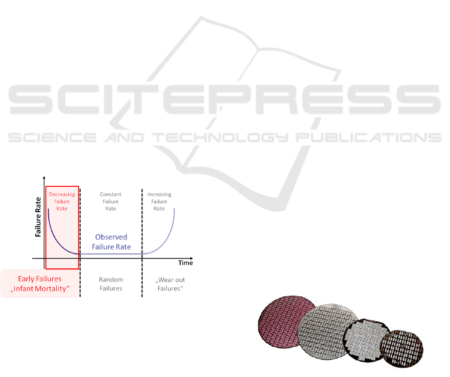
control and high-speed trains. The most delicate pe-

riod for devices is their early lifetime, where fail-

ures represent a high risk as visualized by the bathtub

curve in Figure 1.

Figure 1: The bathtub curve describes the life stages of

semiconductor devices.

The main reason for device failures during the

early life stage comes from the manufacturing pro-

cess. Most of these production failures can be de-

tected with functionality tests, where mainly electri-

cal connectivity is checked. Beside this, further tests

regarding reliability of the devices, are performed. A

generally accepted procedure for investigating relia-

bility issues is the Burn-In (BI) test, where the de-

vices are tested under accelerated stress conditions to

simulate the early lifetime. Due to undesirable side

effects of the BI, like high costs and the need for extra

trained employees, a reduction of devices to be burned

is preferable.

More cost-efﬁcient methods are statistical screen-

ing methods which are capable of detecting potential

early life failures. If a device is suspicious compared

to the majority represents a risk device, so-called

Maverick. Depending on the classiﬁcation power of

the screening method, detected Mavericks are imme-

diately rejected or further investigated, e.g. with the

BI. Due to the development towards sub-micron tech-

nologies, a distinction between reliable devices and

Mavericks becomes increasingly challenging. There-

with, commonly known screening methods do not

work as reliable as before. This opens the need for

advanced methods to solidly detect Mavericks.

A promising approach which is investigated in

the present PhD, is a combination of the Independent

Component Analysis (ICA) followed by the Nearest

Neighbor Residuals (NNR) method (Turakhia et al.,

2005). The idea behind is to perform a data transfor-

mation to reveal masked information by applying the

ICA and afterwards, taking spatial dependencies over

the wafer into account with the NNR (cf. Figure 2).

An ad hoc investigation shows that this is a promising

research direction, but a thorough data analysis has to

precede the ICA to guarantee reliable results.

Figure 2: Wafers can be distinguished e.g. regarding the

size and number of devices, which is considered with NNR.

2 STATE OF THE ART

Commonly, BI testing is performed to detect weak

devices during their early lifetime. Currently, this is

the only fully accepted method among semiconductor

manufacturers to sort out early lifetime failures. Re-

liable screening methods, which can classify devices

Zernig A., Bluder O., Kästner A. and Pilz J..

Device Level Maverick Screening - Application of Independent Component Analysis in Semiconductor Industry.

 2014 SCITEPRESS (Science and Technology Publications, Lda.)

in good ones and Mavericks, consequently reduce the

effort spent on BI. The detection of Mavericks using

screening methods is a cost-efﬁcient, fast and well-

established procedure. Their main target is the identi-

ﬁcation of Mavericks already at an early stage, where-

upon a lot of following tests and production steps can

be skipped which results in a more efﬁcient manufac-

turing sequence. While usual test concepts are de-

signed to detect functionality failures, the intention of

screening methods is the detection of reliability prob-

lems. They are not a question of actual functionality,

but of hidden evidence for failures during early life

stage at customer level. This is then a safety and war-

ranty issue.

2.1 Burn-In Testing

An established method to detect Mavericks is the

Burn-In (BI), where devices are tested over several

hours under increased, but still close to reality, test

conditions, such as high temperature and high sup-

ply voltage. The reliability of this method regarding

detection of early failures is acceptable, but contains

the drawback of high costs, including testing time,

special equipment requiring routine maintenance and

extra trained employees. Moreover, the pre-damage

caused during BI stress implies that the device is no

longer ’virgin’, which introduces an additional reason

to search for other testing methods. Due to the fact

that BI is currently the only fully accepted screen-

ing method among semiconductor manufacturers, the

aim to reduce the number of devices tested with BI

is more realistic than replacing this method. This can

be achieved if the classiﬁcation of good devices and

Mavericks can be performed reliably.

2.2 Part Average Testing

Part Average Testing (PAT) is a standard method,

based on the evaluation of data distributions. These

distributions should be calculated in a robust way,

meaning that the calculated distribution parameters

are insensitive to outliers. Although a variety of dif-

ferent measurements can be used, electrical tests like

diverse current and voltage measurements are prefer-

able. The idea behind is to detect suspicious de-

vices, which indicate some abnormality compared to

the majority of the devices. These devices are then

scrapped and not delivered to the customer. To de-

cide whether a device is suspicious or not, upper and

lower PAT limits, most often calculated on the basis

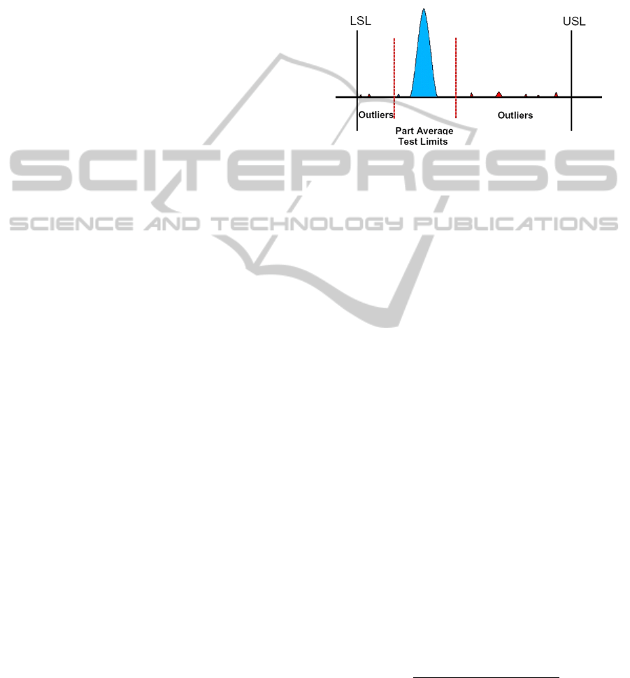
of a normal distribution, have to be set. In generally,

they are tighter than the lower (LSL) and upper (USL)

speciﬁcation limits, see 3. Further, these PAT limits

can be divided into static and dynamic limits. The

main difference between is that the static limits are

calculated once, on the basis of a reasonable amount

of data, and then are further applied for subsequent

wafers. In contrast to this, the dynamic limits are up-

dated for each wafer, which takes the variation be-

tween the wafers into account.

Figure 3: PAT limits, marked in red, are more severe than

the lower (LSL) and upper (USL) speciﬁcation limits.

A further powerful PAT variant is the multivari-

ate PAT. Its focus is the detection of correlated failure

mechanisms of two or more test measurements. Ex-

pert knowledge and experiences with different tech-

nologies are mandatory up to now, to take meaningful

combinations of test measurements for the evaluation

of the multivariate PAT.

2.3 Good Die in Bad Neighborhood

Another commonly used method, known as Good

Die in Bad Neighborhood (GDBN), takes spatial de-

pendencies of devices over the wafer into account.

More accurately, a comparison of each device with its

neighborhood indicates the devices potential risk. It

is known that supposedly good devices surrounded by

bad ones are more likely to fail than those surrounded

by further good ones. An example is given in Figure

4, where a supposed good device is inked out (colored

in gray) because it is surrounded by many bad devices

(marked in black).

Further, it can be observed that devices with the

same risk behavior tend to cluster and those at the

edge of a wafer are more likely to fail due to the man-

ufacturing process of a wafer. The evaluation of good

or bad is done on the basis of the Unit Level Predic-

tive Yield (ULPY) calculation (Riordan et al., 2005),

taking a combination of yield per wafer (local yield)

and yield per lot (stacked yield) into account:

ULPY =

local yield × stacked yield. (1)

Again, devices being outside speciﬁed limits are

inked automatically and rejected in the next produc-

tion step.

ICPRAM2014-DoctoralConsortium

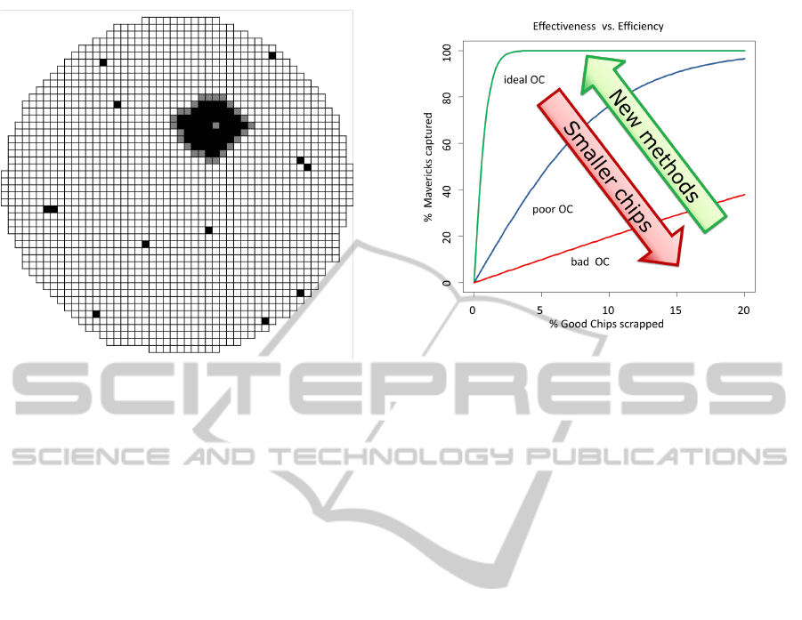
Figure 4: Good devices surrounded by bad devices (marked

in black), are inked out (marked as gray devices).

3 OUTLINE OF OBJECTIVES

Due to the miniaturization of semiconductor devices,

new challenges on screening methods arise. The clas-

siﬁcation in good devices and Mavericks does not

work as accurate as before with screening methods

described in Section 2. Other failure mechanisms ap-

pear or dominate the device failure. To counteract,

advanced screening methods are needed with the aim

to capture as many Mavericks as possible on the ex-

pense of only few good devices (misclassiﬁcations).

To evaluate the classiﬁcation power of a method, this

ratio can be visualized as an operating curve (see Fig-

ure 5). The steeper the ascent of the curve, the more

efﬁcient the method works to separate good devices

and Mavericks. A 100% Maverick detection without

any misclassiﬁcation forms the optimal case.

It is often not the development of a completely

new method which leads to better results, but a combi-

nation of meaningful methods implemented in a rea-

sonable order. It is important to analyze the data basis

which will be used. Further, a transformation is of-

ten necessary to extract special features which lead to

a better understanding of the underlying data. Sec-

tion 5 presents the method of Independent Compo-

nent Analysis (ICA), which is a promising approach

to detect and separate latent information. Afterwards,

post-processing steps can be applied. The Near-

est Neighbor Residuals (NNR) method is proposed,

which takes spatial dependencies over the wafer into

account.

Generally, any combination of data analysis, data

transformation and post-processing methods can lead

Figure 5: With ever smaller devices, a distinction between

good devices and Mavericks becomes challenging. There-

with, the efﬁciency of currently applied screening methods

decreases. New methods are expected to counteract. Con-

sequently, the steeper the operating curve, the higher the

classiﬁcation power of the method.

to advanced screening quality. Therewith, the operat-

ing curve wants to be improved in a way that nearly

all Mavericks can be identiﬁed, including hardly any

misclassiﬁcation.

4 RESEARCH PROBLEM

The intention of this PhD is to develop advanced

screening methods, which can handle the new chal-

lenges on sub-micron devices. As a ﬁrst approach the

work ﬂow schematically displayed in Figure 7 is ex-

amined.

First step is the evaluation and collection of mean-

ingful data for this purpose. Although a variety

of conventional test measurements are done during

the production process, for many applications IDDQ

measurements (Miller, 1999), i.e. measurements of

the power supply current in the quiescent state, are

more informative as e.g. functional voltage tests. De-

pending on the product and the technology, different

numbers of measurements are taken. For the prod-

uct under investigation, 577 IDDQ measurements per

device are collected. When the power consuming el-

ements are switched off, a perfect CMOS has IDDQ

values in the range of some microamperes whereas

higher values indicate a suspicious behavior of one

or more transistors. Sub-micron technologies contain

new failure mechanisms where it is expected that the

currently used screening methods do not work as ac-

curate as before. For instance, smaller devices have

DeviceLevelMaverickScreening-ApplicationofIndependentComponentAnalysisinSemiconductorIndustry

increased leakage current which makes it hard to ﬁnd

a threshold for separating good devices from Maver-

icks. Although, as a ﬁrst attempt, IDDQ measure-

ments seem to be a good choice, also other test mea-

surements or a meaningful combination of them in-

cluded in the calculation may be suitable.

High dimensional data often contain latent infor-

mation, which becomes visible after a meaningful

data transformation, preferably in a 2 or 3 dimen-

sional space for complexity reduction as well as for

visualizing purposes. Afterwards, a separation cri-

terion to divide good devices and Mavericks has to

be found. As a ﬁrst attempt, the ICA is investigated,

which is widely spread e.g. in the ﬁelds of speech

recognition, image processing, text document analy-

sis and biomedical applications. The applicability of

ICA on device data is not that well investigated by

now, but will be evaluated in this PhD.

The aim is to ﬁnd a reliable combination of data

analysis techniques, followed by a meaningful data

transformation (e.g. ICA) and a ﬁnal classiﬁcation

method to detect Mavericks.

5 METHODOLOGY

5.1 Independent Component Analysis

High dimensional data often mask informative fea-

tures which may help to explain an underlying pro-

cess. Independent Component Analysis (ICA) per-

forms a transformation of observable data x, i.e. test

measurements, into a new representation of sources

s. This can be obtained by applying a transformation

matrix A (mainly called mixing matrix) to reveal la-

tent structures. In other words, it is expected that the

measured data are mixtures of sources that want to

be recovered. Mathematically this can be written as

follows:

x = As. (2)

With a simple inversion of the mixing matrix A,

the sources can be calculated:

−1

x = Wx = s. (3)

Due to the fact that both, the sources and the mix-

ing matrix, are unknown, conventionally solving the

equation is not possible. This means that A or W

have to be estimated, leading to approximations for

the sources as well:

s =

Wx. (4)

The idea behind ICA is to separate measurement

data into statistically independent sources. Statisti-

cally independent data contain the most information

because they do not include any redundancy. To

achieve independence, either the non-gaussianity can

be maximized or the mutual information can be min-

imized, as will be outlined in the next section.

5.1.1 Pre-processing for ICA

To perform a reliable ICA, main emphasis lies on data

preparation of the test measurements x. Various pre-

processing methods are available. Commonly used

techniques (Naik and Kumar, 2011) are centering fol-

lowed by whitening. Centering means a subtraction

of the mean from the data. The ensuing whitening

data, x

, is a linear transformation of the measure-

ments whereby x

is uncorrelated with a unit vari-

ance:

Var{x

} = E{x

} = I. (5)

The advantage of whitened measurements is the

reduction of the computational complexity of ICA;

the number of variables to be estimated decreases

from n

for matrix A to





n(n−1)

for a resulting or-

thogonal matrix A

. One method to obtain whitened

data x

is the Singular Value Decomposition with

= VD

−

x, (6)

where V contains the eigenvectors of the covariance

matrix E{xx

} and D is the diagonal matrix of eigen-

values. This modiﬁes the mixing matrix A to an or-

thogonal mixing matrix A

as shown in the following

equation:

= VD

−

As = A

s (7)

with,

E{x

} = E{A

}

= A

E{ss

}

|{z}

= A

= I. (8)

Here, E{ss

} = I can be assumed without loss of gen-

erality because ICA is insensitive to the variance. The

new representation in Equation 7, containing now an

orthogonal matrix A

, has the previously mentioned

advantage of a decrease in complexity. Instead of

the Singular Value Decomposition, also a PCA can

be performed to get uncorrelated data with unit vari-

ance. Geometrically spoken, just a rotation of the ma-

trix has to be found to get the desired independent

data. Therefore, numerical optimization algorithms,

like the gradient descent, can be used and optimized

ICPRAM2014-DoctoralConsortium

using a quantitative measure of non-gaussianity, like

the kurtosis and the Neg-entropy.

Regardless of the distribution of independent ran-

dom variables, based on the central limit theorem,

their sum converges to a Gaussian distribution for a

sufﬁciently large sample size. Conversely, making the

measurements as non-Gaussian as possible will return

these independent sources. This implies the assump-

tion that the sources are independent and further, that

at most one of the measurements is Gaussian. The

usage of the kurtosis as evaluation criterion for non-

gaussianity is quite popular because it is computation-

ally easy to implement. A kurtosis value of zero im-

plies a perfect Gaussian distribution of the underlying

data, whereas a nonzero value indicates a deviation

from the Gaussian distribution. Unfortunately, the

kurtosis is very sensitive to outliers. A more robust

criterion is so-called Neg-entropy which is deﬁned

as a measure of gaussianity, reﬂecting the deviation

of the data from a Gaussian distribution. The disad-

vantage of this method is that the probability density

function of the data has to be known in advance. The

uncertainty about the underlying probability density

function can be compensated using approximations

instead. Another procedure is the Infomax-principle

(Bell and Sejnowski, 1995), which stands for infor-

mation maximization and will be realised by minimiz-

ing mutual information.

Further pre-processing steps, which often result in

dimension reduction techniques, can be performed.

Depending on the data and the application, some

of them use PCA, Projection Pursuit (Friedman,

1987), ﬁltering, stochastic search variable selection

like Bayesian networks and wavelet transformation.

5.1.2 Post-processing after ICA

After the ICA has been performed, the resulting

sources have to be evaluated. This can be again a form

of ﬁltering, e.g. the separation in informative sources

and noise. As a ﬁrst attempt, the NNR method is used,

which takes spatial dependencies of devices over the

wafer into account, see Equation 9. From each device

value, v(x

), the median of the surrounding devices

is subtracted, whereas m and n are dependent on the

neighborhood:

NNR(x

) = v(x

) − med(v(x

i+m

j+n

)). (9)

The size of the neighborhood (8, 24 or more) for

calculating the NNR is a further topic which will be

investigated in this PhD. Previous investigations have

shown that the nearest 24 surrounding devices (m,n =

{−2,−1,1,2}) are a good choice. However, ﬁrst eval-

uations of the NNR on the sources have shown that the

number of surrounding devices taken into calculation

needs to be determined for this project.

Figure 6: To calculate the NNR value for each device (here

marked in gray), just the pass devices are taken into account

because for the electrical fail devices (marked in black) no

value is available. The black square shows the involved de-

vices for a 24-based neighborhood.

As visualized in Figure 6, only pass devices are

considered for the NNR calculation and therefore it

happens that not all surrounding neighbors are avail-

able. In this case it might be useful to consider either

just the given values or other signiﬁcant ones instead.

As a ﬁrst attempt, the gap can be ﬁlled up with de-

vices on the main x-y-directions, starting from device

). Those from the diagonal directions are only

considered if further devices are needed. Addition-

ally, depending on e.g. the distance, weights can be

incorporated.

5.2 Further Considerations

As outlined in Section 5.1.1, various pre-processing

methods are listed, where the most meaningful one

has to be determined to provide a useful starting po-

sition for the ICA method itself. Generally, the num-

ber of sources is unknown, implying that there can be

more sources than measurements (underdetermined)

or vice versa (overdetermined system of equations)

(Naik and Kumar, 2011). For the ﬁrst case, the cal-

culation of a pseudo-inverse is necessary. An applica-

tion can be found e.g. in bio-signal processing, where

the number of electrodes are limited compared to the

active muscles involved. For an overdetermined sys-

tem of equations dimension-reducing pre-processing

steps can be performed, see Section 5.1.1. A re-

duction of the measurements to the number of ex-

pected sources is preferable. For ICA itself, different

MATLAB



packages, like the FastICA (Hyv

arinen

DeviceLevelMaverickScreening-ApplicationofIndependentComponentAnalysisinSemiconductorIndustry

et al., 2001), are available.

6 STAGE OF THE RESEARCH

A ﬁrst and promising approach to detect Mavericks is

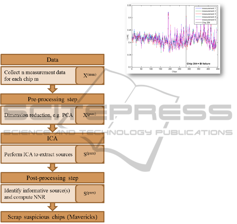
depicted in Figure 7.

Figure 7: The ﬂowchart provides an overview of the pro-

posed way of proceeding.

The proposed way of proceeding starts with the col-

lection of meaningful data, followed by their analysis

and preparation as a pre-processing step for ICA. Af-

ter ICA is performed, the most informative source or

even sources have to be identiﬁed. It is expected that

an additional NNR calculation reveals further latent

information to ﬁnally detect suspicious devices.

6.1 Data and Pre-processing Step

As explained in Section 4, the data under investiga-

tion are 577 IDDQ measurements per device. Figure

8 shows the ﬁrst ﬁve of them. The correlation matrix

C shows strong similarity between the measurements,

Figure 8: Each IDDQ measurement can be visualized as a

signal over all devices. This ﬁgure shows the ﬁrst 5 (su-

perimposed) IDDQ measurements taken from overall 577

available, used as a dimension-reduced basis for the follow-

ing ICA.

with C

i j

> 0.97. Also the PCA has shown, that al-

ready one component explains more than 90 % of the

variability in the measurement data. A dimension re-

duction of the measurement data is recommended as

a pre-processing step. For this, different techniques

will be investigated. With knowledge about the num-

ber of hidden sources in the measurements, the size

of dimension reduction would be determined but this

insight is generally not given. Nevertheless, due to

the high correlations between the measurements, a

huge amount of measurements is at least mathemat-

ically negligible, i.e. contains no additional informa-

tion. This implies the assumption of an overdeter-

mined system, where more measurements are avail-

able than sources expected. As outlined in Section5.2,

a pre-processing step in terms of a dimension reduc-

tion is proposed.

6.2 ICA on 5 IDDQ Measurements

As a ﬁrst attempt, the ICA calculation has been per-

formed on the basis of the ﬁrst ﬁve IDDQ measure-

ments (see Figure 8). The ICA is performed using

the implemented MATLAB function FastICA. The

(5 × 5) mixing matrix A and de-mixing matrix W

are calculated and applied to the measurements (see

Equation 4). The resulting 5 sources are visualized in

Figure 9.

To calculate the mixing matrix, symmetric or-

thonormalization is recommended, which calculates

the sources in parallel. Consider, that for repro-

ducibility the continual ambiguities of scaled and per-

muted sources remain.

ICPRAM2014-DoctoralConsortium

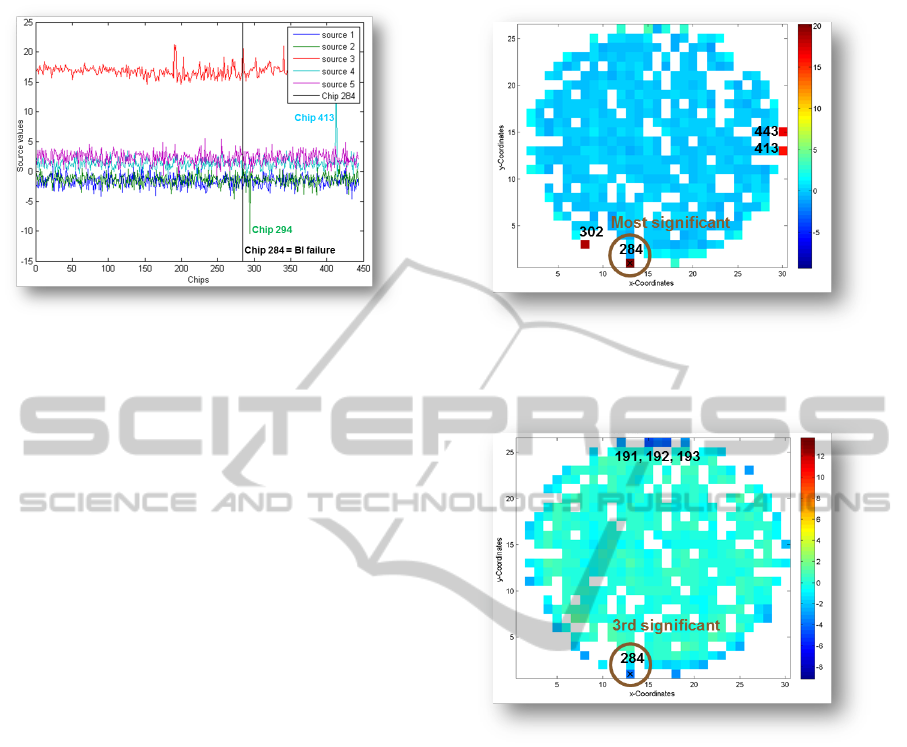
Figure 9: With a quadratic de-mixing matrix W the di-

mension of the resulting sources remains the same. Source

3 (red) is conspicuous compared to the remaining sources

and is therefore assumed to contain the most information.

Source 2 and 4 show one peak each and thus will be inves-

tigated in more detail.

6.3 Post-processing Step

While each of the measurements seems to contain the

same information (optically (see Figure 8) and in-

dicated by high correlations), the ICA transformed

sources show clearly separated signals (see Figure 9).

In contrast to other applications of ICA, e.g. investi-

gations of EEG signals, where the pathway of a stan-

dard signal is known, there is no reference signal for

IDDQ measurements which can be used on a compar-

ative basis. Without the identiﬁcation of one speciﬁc

signiﬁcant source, the NNR is calculated for each of

the ﬁve sources based on 8 as well as on 24 neigh-

bors. Source 3 (see Figure 9, colored in red), which is

conspicuous compared to the remaining sources, even

provides 7 Mavericks from totally 8 detected ones, see

Figure 10 and Figure 11.

Therewith, source 3 seems to include the most in-

formation. Source 4 reveals device 413, whereas this

device has been found with source 3 as well. Source

2 is responsible for the suspicious device 294. NNR8

has to be considered carefully because for devices on

the edge of the wafer, just the available neighborhood

is used, without any gap ﬁlling adaptation (c.f. Sec-

tion 5.1.2). This means that for some NNR calcu-

lations, only few surrounding devices are available,

especially if just an 8-based neighborhood is chosen.

Nevertheless, both ﬁgures show clearly suspicious de-

vices. Device number 284, additionally marked with

a black cross, is extremely suspicious in even both

NNR calculations. Altogether, device 191, 192, 193,

284, 302 and 443 has been detected in source 3, de-

vice 413 in source 3 as well as in source 4 and device

294 is just suspicious in source 2 (see Figure 9). To ﬁ-

Figure 10: The wafer map represents the resulting NNR

calculation on source 3 (see Figure 9) with 8 neighbors

(NNR8). Device 284 is the most signiﬁcant one.

Figure 11: The wafer map represents the resulting NNR

calculation on source 3 (see Figure 9) with 24 neighbors. In

contrast to NNR8, device 284 is the third signiﬁcant one.

nally judge these 8 suspicious devices the results from

the BI study are provided in the next section.

6.4 Investigation of Detected Mavericks

To verify the actual behavior of the previously de-

tected 8 devices during their early lifetime, a BI-study

was performed. Results from Backend and BI testing

reveal that 5 devices (192, 193, 294, 302, 443) failed

in the standard Backend test ﬂow before BI and 2 de-

vices (191 and 284) failed during BI after 2 hours and

12 hours, respectively. Altogether, 7 out of the 8 de-

tected Mavericks failed indeed. Just device number

413 survived the 96h BI test, although it is suspicious

in even two sources. BI survivors are not necessar-

ily devices no longer containing any risk. A lifetime

investigation of these devices may explain their long-

time behavior. Nevertheless, 7 out of 8 is a promis-

DeviceLevelMaverickScreening-ApplicationofIndependentComponentAnalysisinSemiconductorIndustry

ing intermediate result. Further, a more precise in-

vestigation of the BI failure mechanisms is planned to

examine a possible connection between the theoreti-

cally detected Mavericks and their failure type. Pos-

sibly different sources might indicate different failure

mechanisms but this is an open question yet.

Since source 3 itself detects most of the Maver-

icks, an automated detection instead of a visual as-

sessment to identify a meaningful source s, is desired.

Calculating the L

-norm for each source, Equation 10,

reﬂects the applicability at least for source 3, see Ta-

ble 1.

||s

577

∑

j=1

i j

)

1/2

for i = 1,...,5. (10)

Table 1: Calculation of the L

-norm for the 5 sources.

Source L

-norm

1 39.9

2 35.6

3 353.5

4 35.7

5 52.9

Source 3 takes the highest norm value. Unfortu-

nately, rearranging the remaining sources regarding

their descending order of the norm values does not

ﬁt to the observed outcome. Beside source 3, source

2 and 4 detected Mavericks and therewith were ex-

pected to get higher values than source 1 and 5. An

investigation of the sources regarding their four mo-

ments, namely mean, variance, skewness and kur-

tosis, identiﬁes source 3 as the most non-Gaussian

source whereas the remaining 4 sources are close to

noise. Further evaluations have to be done to quantify

this information.

7 EXPECTED OUTCOME

The aim of this PhD is to develop an advanced screen-

ing method to detect Mavericks on sub-micron tech-

nologies with higher integration density, where cur-

rently existing screening techniques do not work as

accurate as before on larger structures. To judge the

classiﬁcation power of the new method, its operating

curve will be evaluated and compared to those of the

already existing screening methods. As an interim re-

sult on the currently investigated data, Table 2 com-

pares the classiﬁcation power between the proposed

method and the commonly used dynamic PAT.

First investigations (see Section 6) have shown

that a meaningful combination of pre- and post-

processing methods improves the performance of

Table 2: Comparison of the classiﬁcation power between

the proposed method (see ﬂowchart in Figure 7) and the

dynamical PAT (DPAT) on the 8 suspicious devices (191,

192, 193, 284, 294, 302, 413, 443).

classiﬁcation proposed method DPAT

correct 7 1

incorrect 1 7

ICA, while ICA itself has free selectable optimization

criteria as well, depending on the application. With

a new improved approach to detect Mavericks, the ef-

fort spend on BI can be reduced and a relevant amount

of time and money can be saved. Additionally, life-

time investigations of Mavericks which survive the

BI may even give information about an appropriate

BI time.

ACKNOWLEDGEMENTS

Special thanks goes to Johannes Kaspar from Inﬁneon

Technologies Austria AG for his valuable discussions

and for being at hand with his expert knowledge any-

time.

This work is funded by the Federal Ministry

for Transport, Innovation and Technology (BMVIT)

funding scheme Talente of the Austrian Research Pro-

motion Agency (FFG, Project No. 839342) and by

Inﬁneon Technologies Austria AG.

REFERENCES

Bell, A. J. and Sejnowski, T. J. (1995). An information-

maximization approach to blind separation and blind

deconvolution. Neural Computation, 7:1129–1159.

Friedman, J. H. (1987). Exploratory projection pur-

suit. Journal of the American Statistical Association,

82:249–266.

Hyv

arinen, A., Karhunen, J., and Oja, E. (2001). Indepen-

dent Component Analysis. John Wiley & Sons.

Miller, A. C. (1999). Iddq testing in deep submicron inte-

grated circuits. In ITC International Test Conference.

Naik, G. R. and Kumar, D. K. (2011). An overview of inde-

pendent component analysis and its applications. In-

formatica, 35:63–81.

Riordan, W. C., Miller, R., and St. Pierre, E. R. (2005). Reli-

ability improvement and burn in optimization through

the use of die level predictive modeling. In Annual

IRPS. 43rd IEEE Annual IRPS.

Turakhia, R. P., Benware, B., Madge, R., Shannon, T. T.,

and Daasch, W. R. (2005). Defect screening using

independent component analysis on iddq. In VTS’05.

23rd IEEE VLSI Test Symposium.