Research on Techniques for Building Energy Model

Dimitrios-Stavros Kapetanakis

, Eleni Mangina

and Donal Finn

School of Mechanical and Material Engineering, University College of Dublin, Dublin, Ireland

School of Computer Science and Informatics, University College of Dublin, Dublin, Ireland

1 STAGE OF THE RESEARCH

Forecasting of building thermal and cooling loads,

without the use of simulation software, can be

achieved using data from Building Energy

Management Systems (BEMS). Experience in

building modelling has shown that data analysis is a

key factor in order to produce accurate results.

Commercial buildings incorporate BEMS to control

the Heating Ventilation and Air-Conditioning

(HVAC) system and to monitor the indoor

environment conditions. Measurements of

temperature, humidity and energy consumption are

typically stored within BEMS. These measurements

include underlying information regarding buildings’

thermal response. Data Mining is utilised to explore

the data, to search for consistent patterns and/or

systematic relationships between variables, and then

to validate the findings by applying the detected

patterns to new subsets of data. The process of data

mining within the current research project consists

of three stages: (1) the initial exploration, (2) model

building or pattern identification with

validation/verification, and (3) deployment (i.e., the

application of the model to new data in order to

generate predictions). The data used for the purposes

of this research project has been gathered from two

commercial buildings, located in Dublin and Cork,

Ireland.

The research described in this paper is at its

initial stage, where an extensive literature review of

building energy modelling has been conducted, the

research plan is defined, the research skills are being

developed and original research work is initiated. In

February 2014, the first year of the three-year

programme will be completed.

2 OUTLINE OF OBJECTIVES

This project focuses on a novel approach for cost-

effective modelling of actual data from commercial

buildings, with models that can be assembled rapidly

and deployed easily. This approach will constitute a

practical research testbed to optimise multiple

objectives related to the buildings’ energy modelling

research area: i) development of a novel approach

for predicting thermal and cooling loads of

commercial buildings; ii) highly accurate predictions

in terms of thermal and cooling loads; iii) scalability

of the new approach to any commercial building and

iv) minimum commissioning and maintenance effort

requirements.

3 RESEARCH PROBLEM

Predictions of building thermal and cooling load can

be obtained using appropriate simulation software.

Building simulation software require detailed

building geometry as well as physical data, such as

construction elements, U-values, etc. in order to

simulate the operation of a building. These

parameters are often unknown, especially for older

buildings, thus introducing rough estimations and

significant commissioning effort in real-world

applications.

An alternative way to forecast these loads is to

take advantage of the data recorder within BEMS.

As already mentioned measurements of temperature,

humidity and energy consumption are the ones

stored within BEMS. Useful information regarding

the thermal response of buildings are contained in

these measurements.

Utilization of measured data can produce

predictions of buildings energy consumption. These

predictions can be used to improve the efficiency of

the HVAC system and hence reduce the amount of

energy consumed. The accuracy of the prediction is

a crucial factor regarding the maximization of

energy savings. This project will attempt to answer

the following research questions:

 Can historical measured data of buildings be

used to predict thermal and cooling load?

 Which is the best methodology to adopt for

model development?

Kapetanakis D., Mangina E. and Finn D..

Research on Techniques for Building Energy Model.

 2014 SCITEPRESS (Science and Technology Publications, Lda.)

 What is the innovation and novelty of the new

model?

 How accurate and scalable is the new model?

 Which are the commissioning requirements of

the new model?

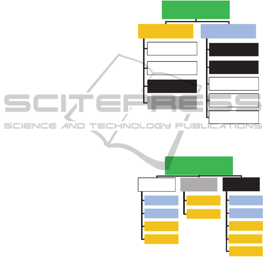
4 STATE OF THE ART

American Society of Heating, Refrigerating and Air-

Conditioning Engineers (ASHRAE) classify

building analytical methods into dynamic and steady

state approaches, as summarised in Figure 1

(ASHRAE, 2009). The difference between steady-

state and dynamic methods is the consideration of

effects such as thermal mass and/or capacitance.

Steady-state methods do not take into account

effects that cause temperature transients.

Conversely, building transient behaviour, which

includes effects such as building warm-up or cool-

down periods, is captured using the dynamic

methods.

Figure 2 illustrates another way to classify the

methods outlined in Figure 1. The key difference is

that the analytical methods are classified based on

the underlying computational methodology rather

than a transient/steady-state demarcation. Three

categories can be observed using this classification,

namely, “White”, “Grey” and “Black” box models.

“White-box” models use physical principles to

calculate the thermodynamics and energy behaviour

of the whole building level or of sub-level

components (Zhao and Magoulès, 2012). The

second category “black-box” models, includes the

data-mining methods, which utilises extensive

measurement of input and output variables in order

to determine correlated relationships between

different variable combinations. The third category

includes models that use both physical and data-

mining methods and are called hybrid or “Grey-box”

models. One can observe that the two different

approaches for classifying the existing

methodologies are two different aspects of the same

issue.

All methods use physical principles or data-

mining techniques and at the same time are either

dynamic or steady-state. This point becomes clearer

while using a colour coding as shown in Figure 1

and Figure 2. White, grey and black colours are used

in Figure 1 to discriminate the white, grey and black

box models. Steady-state methods are coloured with

blue and dynamic methods with orange in Figure 2.

White-box methods do not meet the basic

requirement of this project, which is the use of

historical data and avoidance of detailed building

geometry and construction data.

Figure 1: Categorization of methods used to estimate

building energy performance based on ASHRAE

Handbook (ASHRAE, 2009).

Figure 2: Categorization of analytical methods to estimate

building energy performance based on the underlying

methodology.

Hence, they are not included in a detailed

manner in this research. Furthermore, grey-box

methods combine the use of white- and black-box

methods thus it is reasonable to eliminate them as

well, due to the presence of white-box methods.

Based on the literature review for black-box

methods regression, support vector machine (SVM)

and artificial neural network (ANN) models seem

suitable for generating predictions. Their

Building Energy

Performance

Dynamic Methods

Computer Simulation

(EnergyPlus, DOE-2, etc)

Computer Emulation

(TRNSYS, HVACSIM+)

Artificial Neural Networks

Thermal Networks

Steady State

Methods

Simple linear regression

Multiple regression

Modified degree-day method

Variable-base degree day

method

ASHRAE bin method and

data-driven bin method

Building Energy

Performance

White-box

Models

Variable-base

degree-day

Bin method

Computer

Simulation

Computer

emulation

Grey-box

Models

Thermal

networks

Hybrid models

Black-box

Models

Simple linear

regression

Multiple

regression

Artificial neural

networks

Support Vector

Machine

Genetic

algorithms

ResearchonTechniquesforBuildingEnergyModel

performance and accuracy will be explored further

to determine which one is the most appropriate for

this specific application. Genetic algorithms are

mainly used for optimization rather than forecasting

and for that reason are excluded from deeper

investigation.

An overview of regression, SVM and ANN

methods including their advantages and

disadvantages alongside interesting case-studies

follows.

4.1 Regression Models

The correlation of energy consumption with all

influencing variables can be achieved with the use of

regression models. Development of these empirical

models is based on historical performance data,

which need to be collected prior to the training of

the models. The main objectives of these models are

the prediction of energy usage, prediction of energy

indices and estimation of important parameters of

energy usage. Examples of these parameters are the

total heat capacity, total heat loss coefficient and

gain factors (Zhao and Magoulès, 2012).

In general, regression models can be divided into

simple and multiple regression. Simple regression

models were frequently used in the late ’90s to

correlate energy consumption with climatic

parameters, to obtain building energy behaviour

(Bauer and Scrartezzini, 1998); (Westergren et al.,

1999). Multiple regression analysis is used to predict

a single dependent variable, such as heating demand,

by a set of independent variables, such as shape

factor, building time constant, etc. Multiple

regression shares assumes: linearity of relationships,

same level of relationship throughout the range of

the independent variable, interval or near-interval

data, absence of outliers and data whose range is not

truncated (Catalina et al., 2008). Multiple regression

models can be separated in two major categories,

multiple linear regression models and multiple non-

linear regression models.

4.1.1 Multiple Linear Regression

Multiple linear regression models are also known as

conditional demand analysis (CDA) models and are

usually applied to the building energy forecasting

area (Foucquier et al., 2013). The idea of using the

linear regression for the prediction of energy

consumption in buildings was first proposed by Parti

(1980). The deduction of the energy demand from

the sum of several end-use consumptions added to a

noise term which was the innovation regarding this

method.

The underlying principle of multivariate linear

regression is the prediction of an output variable Y as

a linear combination of input variables (X

,…,X

)

plus an error term ε

(Foucquier et al., 2013).

01122

... , [1, ]

ii pipi

xxin



 





  



(1)

In Equation (1), n is the number of sample data, p is

the number of variables and α

a bias. For instance,

when the output variable is internal temperature the

external temperature, humidity, solar radiation and

lighting equipment can be considered as input

variables (Foucquier, et al., 2013).

Essentially, multiple linear regression models

can be applied both for predicting or forecasting

energy consumption and for data-mining. The main

advantage of these methods is the simplicity of

implementation by non-expert users, since no

parameter needs to be tuned. Nevertheless, multiple

linear regression models imply a major drawback

due to their inability to solve nonlinear problems.

This causes limitations to the flexibility of the

prediction and at the same time presents difficulties

to manage the correlation between several variables.

4.1.2 Multiple Non-linear Regression

Non-linear regression models are of the same basic

form as linear regression models:

(),

iii

fXaY







(2)

The error terms are usually assumed to have a value

of zero, constant variance and to be uncorrelated,

just as for linear regression models. Often, a normal

error model is utilized which assumes that the error

terms are independent normal random variables with

constant variance. The correlation between the input

and output variables can take different forms in

order to fit the available data series. Two examples

of non-linear regression models widely applied in

practice are exponential and polynomial regression

models.

4.1.3 Case Studies

In this section interesting case-studies of regression

models are given. At first, two case-studies which

applied multiple linear regression models are stated

followed by multiple non-linear regression case-

studies.

Lam et al., (2010) developed multiple linear

regression models for office buildings for the five

major climates in China. These models can be used

to estimate the potential energy savings during the

initial design stage when different building schemes

and concepts are being examined. A total of 12 key

ICAART2014-DoctoralConsortium

building variables were identified through

parametric and sensitivity analysis and considered as

inputs in the regression models. More recently,

Aranda et al., (2012) used multiple linear regression

models to predict the annual energy consumption in

the Spanish banking sector. The energy consumption

of a bank branch was predicted as a function of its

construction characteristics, climatic area and energy

performance. Three models were finally obtained.

The first one was used to make predictions for the

whole banking sector, while the rest estimated the

energy consumption for branches with low winter

climate severity (Model 2) and high winter climate

severity (Model 3).

Catalina et al., (2008) worked on the

development and validation of multiple regression

models to predict monthly heating demand for

single-family residential buildings in temperate

climates. The inputs for the regression models were

the building shape factor, building envelope U-

value, window to floor area ratio, building time

constant and climate, which was defined as a

function of temperature and heating set-point. It was

found that quadratic (second-order) polynomial

models were the most appropriate solution for the

problem. In order to validate the models, 270

different scenarios were analysed. The average error

was 2% between the predicted and simulated values.

An update to the aforementioned work was

published by Catalina et al., (2013). A new model to

predict the heating energy demand, based on the

main factors that influence the building heat

consumption, was introduced. Influencing factors

were: the building global heat loss coefficient, south

equivalent surface and difference between indoor set

point temperature and “sol-air temperature”. Once

again, polynomial multiple regression models were

used and a three input model was found to be the

most appropriate for this problem. The model was

tested and demonstrated relativly good accuracy

considering its simplicity and generality. Human

behaviour was also taken into account in the creation

of this model, improving the accuracy of the

predictions.

4.2 Support Vector Machine

The SVM is an artificial intelligence technique that

is usually used to solve classification and regression

problems. It was introduced by Vapnik and Cortes

(1995). As already described, the regression method

is used to characterise a set of data with a specific

equation. The type of the regression equation is

determined by the user. The technique which allows

the demarcation of a set of data in several categories

is called classification. Once again, the

characteristics of each category are given by the

user.

SVM is mainly used with a regression method to

predict the energy consumption of buildings. The

determination of the optimal generalisation of the

model to promote sparsity is the basic principle of

the SVM for regression. A given training dataset

from a nonlinear problem is [(x

),..,(x

)], where

and y

is the input and output space respectively.

The approach to solve this problem is to overcome

the nonlinearity by transforming the nonlinear

relation between x and y in a linear map. To achieve

that, the nonlinear problem must be sent to a high-

dimensional space called the feature space. The aim

is to determine the function f(x) that best fits the

behaviour of the problem as with all the known

regression techniques. A special feature of the SVM

is that it authorises an error or an uncertainty ε

around the regression function (Foucquier et al.,

2013). The form of the f(x) function is the following:

,(() )x





 

(3)

where, Φ represents a variable in the high-

dimensional feature space and <,> is a scalar

product, ω and b are estimated by the following

optimisation problem.



,, ,

min 2

,()

ii i

iii

subject to

yxb

xby























    

 





(4)

where, C is a regularisation parameter, which

introduces a trade-off between the flatness of f(x)

and the maximal tolerated deviation larger than ε,

given by users, ξ

and ξ

are two slack variables,

which allow the constraints to be flexible. In

addition, a kernel function defined as a dot product

in the feature space k(x,x’)= <Φ(x),Φ(x’)> is created

to allow the substitution of the complex nonlinear

map with a linear problem without having to

evaluate Φ(x). Examples of kernel function used in

regression by SVM are the linear [k(x

,x) = x

·x],

polynomial [k(x

,x)= (x

·x+c)

] and radial basis

function (RBF) kernel (Foucquier et al., 2013).

One of the main advantages of the SVM model is

the fact that the optimisation problem is based on the

structural risk minimisation principle. The

minimisation of an upper bound of the

generalization error consisting of the sum of the

ResearchonTechniquesforBuildingEnergyModel

training error is the objective of this method. This

principle is usually encountered at the empirical risk

minimisation which only minimises the training

error. An additional advantage is that with this

method there are fewer free parameters of

optimisation. Application of the SVM technique

requires the adjustment of the regularisation constant

C and the margin ε. At the same time, this

adjustment is one of the hardest steps of this method.

The main drawback of the SVM method is the

selection of the best kernel function corresponding

to a dot product in the feature space and the

parameters of this kernel (Foucquier et al., 2013).

4.2.1 Case Studies

Support vector machine models have been used for

predicting energy consumption in buildings quite

recently. Dong et al., (2005) were the first to

introduce the use of SVM for prediction of the

building energy consumption. The objective of their

work was to examine the feasibility and applicability

of SVM in building load forecasting area. In order to

test the developed SVM model, four commercial

buildings in Singapore were selected randomly as

case studies. The input variables were the mean

outdoor dry-bulb temperature, the relative humidity

and the global solar radiation. The kernel function

used was the radial basis function kernel. The

obtained results were found to have coefficients of

variance less than 3% and percentage of error within

4%.

Li et al., (2009) used the SVM model in

regression to predict hourly building cooling load for

an office building in Guangzhou, China. The

outdoor dry-bulb temperature and the solar radiation

intensity were the input parameters for this model.

Results indicated that the SVM method can achieve

accurate predictions and that it is effective for

building cooling load prediction. A comparison of

the newly developed SVM model against different

artificial neural networks was published by the same

research group later the same year (Li et al., 2009).

The SVM model was compared with the traditional

back propagation neural network, the radial basis

function neural network and the general regression

neural network. All prediction models were applied

at the same office building in Guangzhou, China.

The models were evaluated based on the root mean

square error and mean relative error. Simulation

results showed that these models were effective for

building cooling load prediction. The SVM and

general regression neural network methods achieved

better accuracy and generalisation than the back

propagation neural network and radial basis function

neural network methods.

Hou and Lian (2009) also used a SVM model for

predicting cooling load of a HVAC system in a

building in Nanzhou, China. The performance of the

SVM with respect to two parameters, C and ε, was

explored using stepwise searching method based on

radial-basis function kernel. Actual prediction

results showed that the SVM forecasting model,

whose relative error was about 4%, may perform

better than autoregressive integrated moving average

ones.

4.3 Artificial Neural Networks

Artificial neural network (ANN) is a generic

denomination for several simple mathematical

models that try to simulate the way a biological

neural network (for instance human brain) works.

The main characteristic of such models is the

capability of learning the ‘‘rule’’ that controls a

physical phenomenon under consideration from

previously known situations and extrapolate results

for new situations. This learning process is called

network training. The development of artificial

neural networks is based on the observation of the

biological neural network behaviour (Neto and

Fiorelli, 2008).

Several possible arrangements for artificial

network have been suggested, generating different

and distinct network models, since it is not well

known how a biological neuron is arranged (Fausett,

1994). The feed-forward model is the most known

and simple network arrangement, illustrated in

Figure 3. In this model, the neurons are placed in

several layers. The first one is the input layer, which

receives inputs from outside. The last layer, called

output layer, supplies the result evaluated by the

network. Between these two layers, a network can

have none, one or more intermediate layers called

the hidden layers. The input layer is usually

considered a distributor for incoming signal, hidden

layers are signal classifiers, and output layer is the

organizer of obtained responses (Neto and Fiorelli,

2008).

An important detail about the feed-forward

model is that the neurons of a given layer are only

connected with the previous layer and the next one.

Other possible more sophisticated network

arrangements are possible as well, for instance the

Self-Organising Maps creates models in which the

network itself changes its arrangement during the

training phase.

ICAART2014-DoctoralConsortium

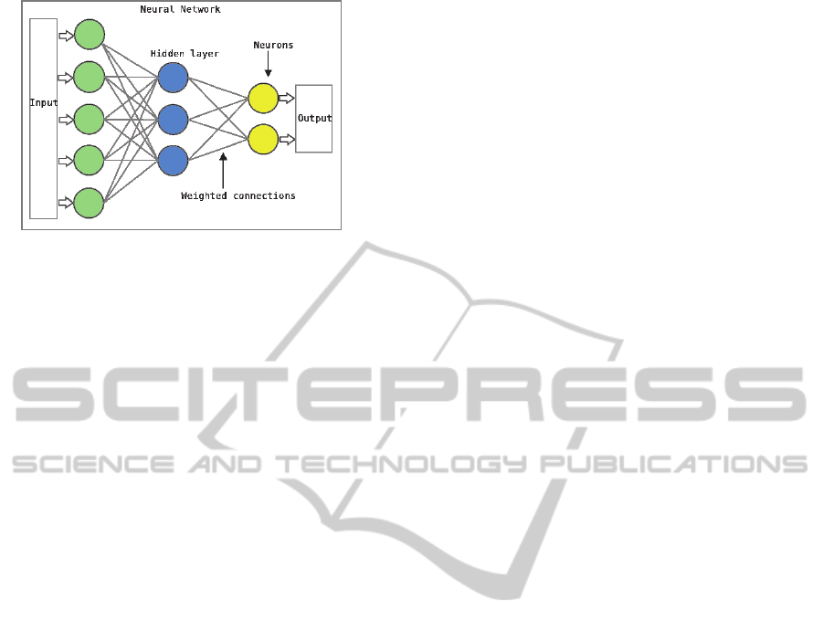
Figure 3: Typical structure of an artificial neural network.

One of the advantages of this method is that it

does not need to detect the potential co-linearity

included in the problem. Another advantage of the

artificial neural networks is its ability to deduce

from data the relationship between different

variables without any assumptions or any postulate

of a model. Moreover, it overcomes the

discretisation problem and is able to manage data

unreliability. This method suggests a large

variability of the predicted variable form (binary 0

or 1, yes/no, continuous value, etc.) and an efficient

simulation time.

Conversely, artificial neural networks are

significantly limited by the fact that a relevant

database should be available in order to be applied.

In fact, it is of vital importance to train the network

with an exhaustive learning basis, which consists of

representative and complete samples. For instance,

samples in different seasons or in different moments

of the day or during weekend or holidays etc. as well

as samples, which contain the same amount of

information. An additional disadvantage of the

artificial neural network is its large number of

undetermined parameters, for which there are no

rules to determine (Foucquier et al., 2013).

4.3.1 Case Studies

Artificial neural networks have been applied by

researchers to analyse various types of building

energy consumption, such as heating and cooling

load, under different conditions.

Kalogirou et al., (1997) implemented back

propagation neural networks at an early design stage

in order to predict the required heating load of

buildings. The network was trained based on 250

known cases of heating load, varying from large

spaces of 100 m

floor area to very small rooms.

Input data included the areas of windows, walls,

partitions and floors, the type of windows and walls,

classification on whether the space has a roof or

ceiling, and the design room temperature. Another

artificial neural network for the estimation of daily

heating and cooling loads was developed by the

same group of researchers (Kalogirou et al., 2001).

A multi-slab feed-forward architecture having 3

hidden slabs was used and each slab comprised of 36

neurons. The accuracy of this network was within

the acceptable level (relative error 3.5%).

The predictions of an artificial neural network

can be made on an hourly basis as well. Gonzalez

and Zamarreno (2005) were based on a special kind

of artificial neural network, which feeds back part of

its outputs, to predict the hourly energy consumption

in buildings. The network was trained by means of a

hybrid algorithm. The inputs of the network were

current and forecasted values of temperature, the

current load and the hour and the day. The achieved

results demonstrated high precision.

The performance of adaptive ANN models that

are capable of adapting themselves to unexpected

pattern changes in the incoming data was evaluated

by Yang et al., (2005). Two adaptive models were

proposed and evaluated, accumulative training and

sliding window training. These models can be used

for real-time on-line building energy prediction.

Moreover, they used both simulated (synthetic) and

measured datasets. When synthetic data was used

the two models appeared to have equal performance

in terms of coefficient of variation (CV). On the

other hand, when real measurements were used the

sliding window training performed better than

accumulative training, CV of 0.26 compared to 2.53

respectively.

More recently, Ekici and Aksoy (2009) used an

ANN to predict building energy needs benefitting

from orientation, insulation thickness and

transparency ratio. A back propagation network was

preferred and available data were normalised before

being presented to the network. The calculated

values compared to the outputs of the network gave

satisfactory results with a deviation of 3.4%.

Dombayci (2010) developed an artificial neural

network model in order to forecast hourly heating

energy consumption of a model house. The hourly

heating energy consumption of the model house was

calculated with degree-hour method. The model was

trained with heating energy consumption values of

years 2004–2007 and tested with heating energy

consumption values for the year 2008. Best estimate

was found with 29 neurons and a good coherence

was observed between calculated and predicted

values.

A comparison between detailed model

simulation and artificial neural network for

ResearchonTechniquesforBuildingEnergyModel

forecasting building energy consumption was

published by Neto and Fiorelli in 2008. EnergyPlus

was used as the model based on physical principles.

Results of this study indicate that EnergyPlus

consumption forecasts present an error range of

±13% for 80% of the tested database. Major source

of uncertainties in the detailed model predictions are

the improper evaluation of lighting, equipment and

occupancy schedules. The artificial neural network

model results had an average error of about 10%

when different networks for working days and

weekends were implemented. The outcome of this

study was that both models are suitable for energy

consumption forecast.

In the same year Aydinalp-Koksal and Ugursal

(2008) compared the use of neural network against

conditional demand analysis (CDA) and engineering

approaches for modelling the end-use consumption

in the residential sector in Canada. The prediction

performance and the ability to characterise the

consumption of the aforementioned methods were

compared in this study. The results indicated that

neural networks and CDA are capable of accurately

predicting the energy consumption in the residential

sector as well as energy simulation programs.

Moreover, the effects of socio-economic factors

were estimated using the neural network and the

CDA model, where possible. Neural network model

was proved to have higher capability of evaluating

these effects compared to the CDA model.

5 METHODOLOGY

Based on the methodologies described earlier new

models will be developed taking account of the key

principles outlined in the objectives. In order to

achieve this, the sequence presented below will be

followed:

 Acquisition of real measured data of a

commercial building (testbed 1) from installed

sensors;

 Data analysis;

 Development of the new models;

 Improvement of models accuracy;

 Evaluation of new models based on accuracy and

on-line training capability;

 Selection of the most suitable model;

 Examination of model scalability with the use of

another commercial building (testbed 2);

 Determination of commissioning and

maintenance effort for the implementation of the

model.

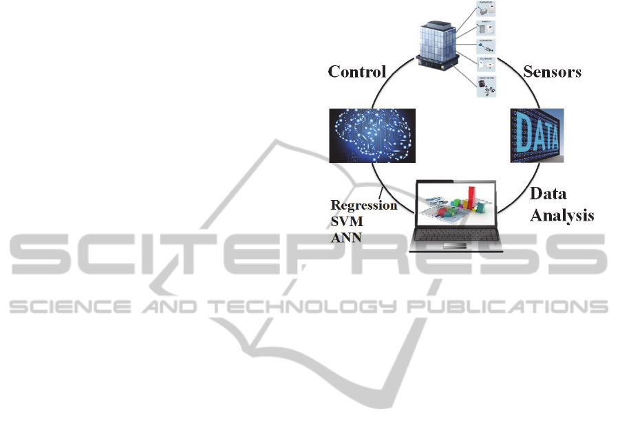
The methodology that is described in this

sequence is also illustrated in Figure 4.

Figure 4: Development of methodology.

The first step of this methodology is to acquire as

much data as possible from BEMS already installed

in a commercial building. Afterwards, data analysis

is employed to replace missing data and correlate

variables to obtain a complete and comprehensive

dataset. The ultimate goal of this data mining

process is to assist with building load prediction,

where incomplete data is available.

Data Mining is utilised to explore the data, to

search for consistent patterns and/or systematic

relationships between variables, and then to validate

the findings by applying the detected patterns to new

subsets of data.

In order to determine the new model the

selection of the optimum model between regression,

SVM and ANN models is required. Different

multiple regression models will be developed

alongside numerous SVM models and several

architectures of ANN and tested in order to reach the

optimum one. The chosen model amongst the

aforementioned will be selected based on its

accuracy and tested for its ability to train on-line.

The scalability of the model will be the next

thing under examination. Data from a second

commercial building will be introduced to the model

and its ability for accurate predictions will be tested

once again.

Finally, commissioning and maintenance effort

for the implementation of the new model will be

determined. Hence, the model will be evaluated

based on its ability to meet the necessary

requirements.

ICAART2014-DoctoralConsortium

6 EXPECTED OUTCOME

The expected outcome of this project is the

development of a novel whole-building energy

model. The model will take advantage of historical

measured data of commercial buildings in order to

generate accurate prediction of heating and cooling

load. Data analysis will be one of the milestones of

this project, since usually measurements include

missing values due to equipment malfunction,

maintenance, etc. An efficient method of dealing

with missing values related with acquired datasets

will be the first outcome of the project.

Once a comprehensive dataset is obtained, the

most suitable methodology for this application is

going to be selected between regression, SVM and

ANN models. An evaluation of the developed

models will take place based on the accuracy of each

model and its ability to train on-line or not. The

selection of the most appropriate model will be the

second outcome.

After the selection process, the chosen model

will be evaluated based on its scalability. The ability

of forecasting heating and cooling loads of two

different given building within the same level of

accuracy will be the criterion. If the chosen model

does not have the desired scalability, then another

model will be selected from the previous procedure

and examined based on its scalability. Finally, the

effort required for commissioning and maintenance

of the model should be as little as possible. The final

outcome should be a scalable model with minimum

commissioning and maintenance requirements.

Ideally, this novel approach of estimating the

thermal and cooling load of commercial buildings

could be implemented to the control of the BEMS.

In this way, the efficiency of the HVAC systems of

the building could be improved reducing the energy

consumption at the same time. This will also lead to

a reduction of the energy cost of commercial

buildings.

REFERENCES

Aranda, A. et al., 2012. Multiple regression models to

predict the annual energy consumption in the Spanish

banking sector. Energy and Buildings, Volume 49, pp.

380-387.

ASHRAE, 2009. Energy Estimating and Modeling

Methods. In: ASHRAE Handbook-Fundamentals.

Atlanta: American Society of Heating, Refrigerating

and Air-Conditioning Engineers, Inc., pp. 32.1-32.33.

Aydinalp-Koksal, M. & Ugursal, V. I., 2008. Comparison

of neural network, conditional demand analysis, and

engineering approaches for modeling end-use energy

consumption in the residential sector. Applied Energy,

85(4), pp. 271-296.

Bauer, M. & Scrartezzini, J., 1998. A simplified

correlation method accounting for heating and cooling

loads in energy-efficient buildings. Energy and

Buildings, 27(2), pp. 147-154.

Catalina, T., Iordache, V. & Caracaleanu, B., 2013.

Multiple regression model for fast prediction of the

heating energy demand. Energy and Buildings,

Volume 57, pp. 302-312.

Catalina, T., Virgone, J. & Blanco, E., 2008. Development

and validation of regression models to predict monthly

heating demand for residential buildings. Energy and

Buildings, Volume 40, pp. 1825-1832.

Dombayci, A., 2010. The prediction of heating energy

consumption in a model house by using artificial

neural networks in Denizli–Turkey. Advances in

Engineering Software, 41(2), pp. 356-362.

Dong, B., Cao, C. & Lee, S. E., 2005. Applying support

vector machines to predict building energy

consumption in tropical region. Energy and Buildings,

37(5), pp. 545-553.

Ekici, B. B. & Aksoy, U. T., 2009. Prediction of building

energy consumption by using artificial neural

networks. Advances in Engineering Software, 40(5),

pp. 356-362.

Fausett, L., 1994. Fundamentals of neural networks:

architectures, algorithms, and applications. Upper

Saddle River, NJ, USA: Prentice-Hall, Inc.

Foucquier, A. et al., 2013. State of the art in building

modelling and energy performances prediction: A

review. Renewable and Sustainable Energy Reviews,

Volume 23, pp. 272-288.

González, P. A. & Zamarreño, J. M., 2005. Prediction of

hourly energy consumption in buildings based on a

feedback artificial neural network. Energy and

Buildings, 37(6), pp. 595-601.

Hou, Z. & Lian, Z., 2009. An Application of Support

Vector Machines in Cooling Load Prediction. Wuhan,

s.n., pp. 1-4.

Kalogirou, S. A., Neocleous, C. C. & Schizas, C. N., 1997.

Building heating load estimation using artificial neural

networks. s.l., s.n., pp. 1-8.

Kalogirou, S., Florides, G., Neocleous, C. & Schizas, C.,

2001. Estimation of Daily Heating and Cooling Loads

Using Artificial Neural Networks. Napoli, Clima

2000.

Lam, J. C., Wan, K. K. W., Liu, D. & Tsang, C. L., 2010.

Multiple regression models for energy use in air-

conditioned office buildings in different climates.

Energy Conversion and Management, 51(12), pp.

2692-2697.

Li, Q. et al., 2009. Applying support vector machine to

predict hourly cooling load in the building. Applied

Energy, 86(10), pp. 2249-2256.

Li, Q. et al., 2009. Predicting hourly cooling load in the

building: A comparison of support vector machine and

ResearchonTechniquesforBuildingEnergyModel

different artificial neural networks. Energy Conversion

and Management, 50(1), pp. 90-96.

Neto, A. H. & Fiorelli, F. A. S., 2008. Comparison

between detailed model simulation and artificial neural

network for forecasting building energy consumption.

Energy and Buildings, 40(12), pp. 2169-2176.

Parti, M. & Parti, C., 1980. The total and appliance-

specific conditional demand for electricity in the

household sector. Bell Journal of Economics, Volume

11, pp. 309-321.

Vapnik, V. & Cortes, C., 1995. Support-Vector Networks.

Machine Learning, Volume 20, pp. 273-297.

Westergren, K.-E., Högberg, H. & Norlén, U., 1999.

Monitoring energy consumption in single-family

houses. Energy and Buildings, 29(3), pp. 247-257.

Yang, J., Rivard, H. & Zmeureanu, R., 2005. On-line

building energy prediction using adaptive artificial

neural networks. Energy and Buildings, 37(12), pp.

1250-1259.

Zhao, H.-X. & Magoulès, F., 2012. A review on the

prediction of building energy consumption. Renewable

and Sustainable Energy Reviews, 16(6), pp. 3586-

3592.

ICAART2014-DoctoralConsortium