
A Network Dispersion Problem for Non-communicating Agents
Martin N. Simanjuntak
Warwick Business School, The University of Warwick, Coventry CV4 7AL, U.K.
1 THE RESEARCH PROBLEM
Is coordination possible when agents are unable to
communicate? This is an abstract problem that can
only be made concrete by the specification of a well-
defined goal of the coordination processes. For
example, the problem of rendezvous of two or more
agents on a network is one that has been extensively
studied for non-communicating agents (see, e.g.,
Alpern and Gal, 2003). A less studied and more
recent problem is the opposite one of achieving
spatial dispersion. If there are n agents at
k
locations, we say that they are dispersed if no
location has more than one agent (this requires of
course that
k is at least n ). In the case of nk
(the main case studied here), dispersion implies
coverage, that is, every location has at least one
agent.
Alpern and Reyniers (2002) initiated the study of
spatial dispersion of agents in the context of non-
communicating agents who could move between any
two locations, based only on the knowledge of the
populations at all locations.
The research problem addressed in this paper is
to see how the problem of Alpern and Reyniers
changes if a network (graph) structure is imposed on
the set of locations: An agent only knows the
population at his current node (location) and he can
only stay still or move to an adjacent node. He can
see the number of arcs at his node, but if he moves
he must choose among them equiprobably. As we
are dealing with non-communicating agents with
limited amount of global knowledge, we shall limit
our discussion to simple and myopic strategies. In
particular, our agents adopt common (Markovian)
stunted random walk strategy, completely specified
by the probability
p
of staying still for another
period at the same node. Given such strategies, how
long will it take, on average, for the agents to
achieve dispersion? The optimization can be simply
with respect to
,
p
or with respect to ,
i
p where
i
is
the population at the agent’s current node. For
example, in the trivial case of a network with two
nodes, where both agents start at the same node, the
optimal value of
p
is ½ and the expected time to
dispersion is
2T
periods.
We shall introduce the network dispersion
problems by way of the following illustration.
Suppose that at 11am the guards at the Louvre have
called a wildcat strike for noon. The Louvre by law
must be kept open. We know that there are n
rooms, but at short notice we don’t have a map. We
can hire in an hour n guards, but they may speak
different languages and will not be able to
communicate with each other. We have a single
broadcasting line for communication to all these new
guards, but we cannot give different guards different
instructions as we do not even know their names.
Once all the rooms have guards, we can broadcast a
command to stay still. To keep things simple, we
assume that time is divided into periods and that
each guard visits only one location in each period.
All we can broadcast is a single number
p , the
probability that a guard should stay still for that
period. We want this to occur before the word gets
out that this is a good time to steal a painting, so we
want to minimise the expected time to reach full
coverage of all the rooms. How can we define a
common strategy for the guards that is simple yet
still effective? And how fast on average will they
arrive at the goal of getting as dispersed as possible?
2 STATE OF THE ART
Our agents are not the smart rational individuals that
are normally assumed in game theory models.
Instead, this type of agent is normally studied in the
domains of Artificial Intelligence and Biology
(social animals). Therefore we found that the works
that are most relevant to our study comes from those
two research communities.
After the paper of Alpern and Reyniers (2002),
Grenager et al. (2002) generalized the specific
problem to a general class of dispersion games. In
this type of games, agents win positive payoff only
66
N. Simanjuntak M..
A Network Dispersion Problem for Non-communicating Agents.
Copyright
c
2014 SCITEPRESS (Science and Technology Publications, Lda.)

when they choose distinct actions. Problems with
similar characteristics have been studied in many
research areas. Here we list some of them:
1. Load balancing: a set of tasks is to be
assigned to a set of machines, and to minimise
the overall processing time, the load need to be
distributed as evenly as possible (see, e.g.,
Azar et al., 1999).
2. Niche selection: this problem has been studied
in economics as well as in ecology. In
economics, it models a situation in which
producers wish to occupy one of a number of
different market niches, and they prefer to
occupy niches with fewer competitions. A few
examples are the Santa Fe problem (Arthur,
1994) and the class of minority games (Challet
and Zhang, 1997). In ecology, this problem is
also called habitat selection, and an example of
this is how animals choose feeding patches
with low population density with respect to
food supply (see, e.g., Houston and
McNamara, 1997). In particular, Fretwell and
Lucas (1969) introduced the equilibrium notion
of the ideal free distribution for habitat
distribution in birds. That is a particular
analogue of our notion of dispersion, where
some nodes have greater capacity (habitat is
more supportive of foragers).
3. Congestion games: proposed initially by
Rosenthal (1973), in this class of games
individuals seek facilities or locations of low
population density, due to the monotonically
increasing cost of using the facilities. One of
the subclasses of congestion games that has
received significant attention is routing games,
in which a set of players in a network choose
the route with low congestion level (see, e.g.,
Qiu et al. 2003).
4. Multi-agent area coverage: a team of agents
seek to cover an entire area (which may or may
not be known a priori), and therefore it is
preferred that each agent covers different part
of the area. This problem has been studied in
several research communities, including
robotics/agents, sensor networks, and
computational geometry. For a recent survey in
the fields of robotics, see Galceran and
Carreras (2013).
3 OBJECTIVES
Given a graph
G
with k nodes, we want to see
which (Markovian) stunted random walk strategies,
if simultaneously adopted by all agents, lead to the
least expected time
T
to dispersion? In all the
problems considered, the same optimization
criterion is used. We consider both (i) a random
initial placement of the n agents onto the
k nodes
of
,G and (ii) an initial placement of all the agents
onto a single node
j
of
.G
In the latter case, it is of
interest to see where the best place to introduce the
agents is.
We also will consider two types of stunted
random walk strategies, and compare them. First, a
simple type, where there is a common parameter
p
representing the probability of staying still for the
next period. Second, a probability vector
p
in which
i
p (the i-th entry in the vector) gives the probability
of staying still (rather than randomly moving) that
depends on the number
i
of agents currently at your
node (called the agent population of the node).
A conjecture of Alpern and Reyniers (2002) in a
related context says that if you are alone at your
node then you should not move and no one should
move to your node. While this might work in the
context of a complete graph, it clearly fails on the
line graph
.
n
L In the case when there are many
agents at node 1 and one agent at node 2, the ones at
node 1 could never disperse. However the weaker
property of setting
1
1p
seems to hold for some
graphs, which does not have the added assumption
that no one goes to a node with current population of
1.
Our objective is to determine the minimum
dispersal time and optimal levels of
p
or of
,p
for
several classes of networks, including line networks
,
n
L cycle networks ,
n
C and complete graphs .
n
K
We also wish to compare on
n
L the efficiency of an
initial placement of all agents at a node
,
j
as
j
varies. It would seem likely that it is better to place
them as close as possible to the centre.
From now on we assume that the graphs we
consider have n nodes and that there are n agents.
4 METHODOLOGY
To evaluate the expected dispersal time T on a
graph
G
as a function of the stationary probability
p
(or of the vector
1
( ,..., )
n
pp
p ) we use two
distinct methodologies. For small graphs (small n ),
we use the theory of absorbing time for Markov
chains. The states of the chain are the population
ANetworkDispersionProblemforNon-communicatingAgents
67

distributions, allowing for symmetry. For example,
the state
123
,,mm m says there are
1
m
agents at
node 1,
2
m at 2 and
3
m at 3. By symmetry of nodes
1 and 3 we may assume
1
m
is at least as large as
3
.m Thus the states when
3
GL are
3, 0, 0 ,
2,1, 0 ,
2, 0,1 ,
1, 2, 0 ,
0,3, 0 , and the absorbing
(dispersed) state
1,1,1 . In general, the set
n
S of all
states for the network dispersion problem on
n
L can
be described as follows, where
12 1
1
[, ,..., ]: ,
n
nnni
i
Ssmmmmmmn
When
n
is larger than 3, the number of states in
this type of analysis becomes too large for
Markovian analysis, so another methodology is
needed – simulation. We use the software
application Mathematica to simulate the movement
of agents adopting a common p-strategy, and
minimize the dispersal time numerically. For
purposes of comparison, and to check our simulation
program, we analyse the line graph
3
L both ways.
5 STAGE OF RESEARCH –
RESULTS SO FAR
5.1 Markovian Analysis for L
3
We first analyse the problem on a line graph
3
L of
three nodes using Markov chain theory. We define
six states in
3
L problem (up to symmetry):
1
[3, 0, 0],s
2
[2,1,0],s
3
[2,0,1],s
4
[1, 2, 0],s
5
[0,3,0],s and the absorbing state,
6
ˆ
[1,1,1].ss
We do not put any restrictions on the movement of
the agents, other than if an agent chooses to move in
the next period, then they can only move to a node
adjacent to the current node. This implies that each
state in the Markov chain is accessible from any
other states (albeit accessing a particular state could
take more than one or two steps). A Markov chain
with this characteristic is defined as an absorbing
Markov chain, for which a set of theoretical
formulas has been devised to calculate the expected
time to absorption. In this subsection we follow the
procedures explained in Grinstead and Snell (1997)
to find the time to absorption, or more generally, the
expected dispersal time
.T
Definition (Absorbing Markov Chain) (Grinstead
and Snell, 1997): A Markov chain is absorbing if it
has at least one absorbing state, and if from every
state it is possible to go to an absorbing state (not
necessarily in one step).
In an absorbing Markov chain, the probability of
absorption is 1. This means that for our problem, the
process will eventually end at the absorbing state
ˆ
[1,1,1].s
However, we have two special situations
in which our Markov chain is no longer absorbing. It
is if the value of p, the probability of staying still, is
set to either 0 or 1. If p is set to 0, three of the states
([3, 0,0], [2,0,1], and [0,3,0]) cannot access
ˆ
s
,
whereas if
p is set to 1, then all states become
absorbing states, and thus do not communicate with
each other. Therefore, the absorbing Markov chain
theory only applies when we restrict the range of
p
as
01.p
For the case of 0p , as well as
1p
, we shall describe another approach separately
in the following section.
5.1.1 Simple Stunted Random Walk
We begin by considering simple strategies based on
a single probability
p for staying still. In each
period, each agent independently decides to remain
at his current node or to move. If he chooses to
move, he observes the number of arcs from his node
and choses to move along them equiprobably. In the
case of a line graph this is elementary: if at an end,
he moves to the unique adjacent node; otherwise, he
randomly moves left or right. We wish to find the
strategy parameter
s
pp
that minimises the
expected time
,TTsp
to reach the unique
absorbing state
ˆ
[1,1,1]s
from the state s. We
denote this minimum time by
,.TTsp
Sometimes we wish to start from a random state,
where each state occurs with its probability of
occurring from a binomial distribution, that is, if
each of the n agents was randomly placed on one of
the n nodes. In this case the expected absorption
time is called
,TTrp
, where r stands for the
random initial state. To calculate
,T we first define
the transition matrix
Q
comprising a set of
transition probabilities between all states in the
chain.
In the transition matrix Q,
ij
q
gives the transition
probability of moving from state
i
s
to state
j
s
in one
step. For example, for the transition probability from
3
s
to
2
,
s
we have
2
32
(1 )pqp
, which means
ICAART2014-DoctoralConsortium
68

that, if the current state
3
[2,0,1]s , then we can
reach the state
2
[2,1,0]s in the next period if the
two agents at the left stay still
2
(),p
and the agent at
the right moves to the middle
(1 ).p
We then construct the matrix
Q
(a submatrix of
Q ), which is a 5-by-5 matrix consisting of the
transition probabilities of all the transient states (all
states except
ˆ
s
), that is, the upper left submatrix.
We wish to determine the column vector
pττ
whose i-th entry is
,
ii
Ts p
, the
expected dispersal time from state
i
s
. Then we can
minimise this expression, for each
,i
with respect to
the parameter
.p According to the theory of
absorbing Markov chains (Grinstead and Snell,
1997), the vector is given by the formula:
1
τ IQ c
where
I is the identity matrix, and c is a column
vector, of which all of the entries are 1. In the simple
stunted random walk strategy, the value of
τ
as a
function of
p is:
Before we present the results for optimal stunted
random walk strategy, we now come back to the two
specials situations in which the chain is not
absorbing. It is when the value for
p is either 0 or 1.
For
1,p
it is quite obvious that if no agent moves,
then we will never reach the equidistribution state.
We then focus on the case of
0.p
Let us see the
value for the transition matrix in this case:
From the transition matrix above, we can see that
the equidistribution state
6
ˆ
()
s
s is only accessible
(not necessarily directly) from two states,
2
s
and
4
,
s
meaning that it is only possible to achieve
dispersal if the agents start from state
2
[2,1,0]s or
4
[1, 2, 0].s
From
4
,
s
if all agents move, the one at
the left end must move to the center. The two at the
center equiprobably move to different ends
(reaching state
6
s
) or to the same end (state
2
s
). We
can now simplify the chain into the following
diagram:
Figure 1: The state transition diagram for
3
L
with. 0.p
Now we can calculate the expected time to reach
s6 from those two states:
11 12 13 14 15 16
21 22 23 24 25 26
31 32 33 34 35 36
41 42 43 44 45 46
51 52 53 54 55 56
61 62 63 644 65 66
()
qqq q qq
qqq q qq
qqq q qq
p
qqq q qq
qqq q qq
qqqq qq
Q
11 12 13 14 15
21 22 23 24 25
31 32 33 34 35
41 42 43 44 45
51 52 53 54 55
qqqqq
qqqqq
qqqqq
qqqqq
qqqqq
Q
65432
6432
2
32
54 32
42
5432
6432
432
432
8 128 22 58 10 1
38 4 3 1
16 1
3( 1) 2 3 2 1
8834891
()
3( 1) 8 4 1
8402636212
38 4 3 1
41615121
32
pppppp
pp pp pp
pp
pppp
pp ppp
p
ppp pp
ppppp
ppppp
pppp
ppppp
τ
1
000010
000100
000010
11
0000
22
13
000
(0)
0
44
000001
p
Q
24
44
(,0)1 (,0)
11
(,0) (2 (,0)) 1
22
Ts Ts
Ts Ts
ANetworkDispersionProblemforNon-communicatingAgents
69

which gives the values
2
(,0) 4Ts and
4
(,0) 3.Ts These values happen to be the optimal
expected time from
2
s
and
4
,
s
as the expected times
for other values of p are bigger than 4 and 3,
respectively. In other words, for
2i or
4,
the
minimising value of
p is 1. For other values of ,i
we minimise the expressions for each row of the
vector τ with respect to
p in (0,1).
We can now list our results on the optimal
expected time using simple stunted random walk
strategy as well as the accompanying p values
(Table 1).
Table 1: Optimal expected times for simple stunted
random walk on L
3
.
Starting state
T
p
Random, r 4.2274 0.2332
s
1
= [3,0,0] 6.2125 0.2415
s
2
= [2,1,0] 4 0
s
3
= [2,0,1] 5.3333 0.5000
s
4
= [1,2,0] 3 0
s
5
= [0,3,0] 5.2836 0.3219
We can see that on average, the agents can
achieve their goal the fastest by starting from state
4
,
s
and setting their probability of staying still p as
zero. It is unlikely, though, that setting
0p
would provide an optimal solution in larger line
graphs. This occurrence is mainly due to the
simplicity of the graph. Other solutions that give
good values are from random placement
( 4.2274)T and when all agents start at the middle
node
( 5.2836)T . These values provide us with a
benchmark for checking the validity of our
simulation techniques for the
3
L .
5.1.2 Compound Stunted Random Walk
In the compound stunted random walk model on
3
,L we allow the stationarity probability (of
remaining at the current node) to depend on the
population of agents at that node. That is, if the total
number of agents at your node is ,i then stay at that
node with probability
;
i
p otherwise move randomly
to a neighbouring node. In this case we get a
transition matrix
Q
whose elements are functions
of the three probabilities
1
,p
2
,p and
3
.p
For example the transition probability
from
[1, 2, 0] to [1,1,1] is given by
12 2 12 2
21 1/2 1 .pp p pp p The agent
who is alone at the left must stay still, which
happens with probability
1
p , and one of the two at
the middle must move while the other one stays,
which happens with probability
22
21pp .
Finally, the one who moves must move to the
unoccupied end (probability ½ in a random walk).
Then, using the same formula for τ as in the
previous section, we get dispersal times from state
i as a function of
1
,p
2
,p and
3
.p Minimising
these five expressions (and an average expression
for the top line corresponding to the random start
r )
with respect to varying all three probabilities gives
the solution to the minimum problem as seen in
Table 2. Note that except for the two states
discussed separately above, we have that the optimal
value of
1
p is 1. This says that if you are the only
agent at your node, stay still. This is similar to a
conjecture in Alpern and Reyniers (2002) for a
related problem, that singleton agents should stay
still, and other agents should not move to their
locations.
Table 2: Optimal expected times for compound stunted
random walk on L
3
.
Starting
state
T
1
p
2
p
3
p
Random, r 3.4006 1.0000 0.4646 0.1331
s
1
= [3,0,0] 5.3672 1.0000 0.4987 0.0831
s
2
= [2,1,0] 4 0 0 any
s
3
= [2,0,1] 2.7405 1.0000 0.5696 0.0537
s
4
= [1,2,0] 3 0 0 any
s
5
= [0,3,0] 4.3076 1.0000 0.4973 0.1425
5.2 Simulation Analysis for L
3
For line graphs
n
L with large n (3),n the
Markov solution technique is not feasible, so we will
use simulation. To check the validity of the
simulation technique, we apply it also to the solved
case of
3
L . We shall see that we get a close fit to the
Markovian solution. For the simulation programme,
we modify the state formulation, by numbering the
three agents. The state
,,ijk
says that agent 1 is at
node i, agent 2 is at node j and agent 3 is at node k.
For example, state
1, 3, 2
. The first entry, 1, shows
that the first agent is at location 1. The second entry,
3, means that the second agent is at location 3, and
the final entry means the third agent is at location 2.
So this state is actually one of our absorbing states,
ICAART2014-DoctoralConsortium
70
in which every agent choose distinct locations.
There are in total 3
3
= 27 states in this formulation.
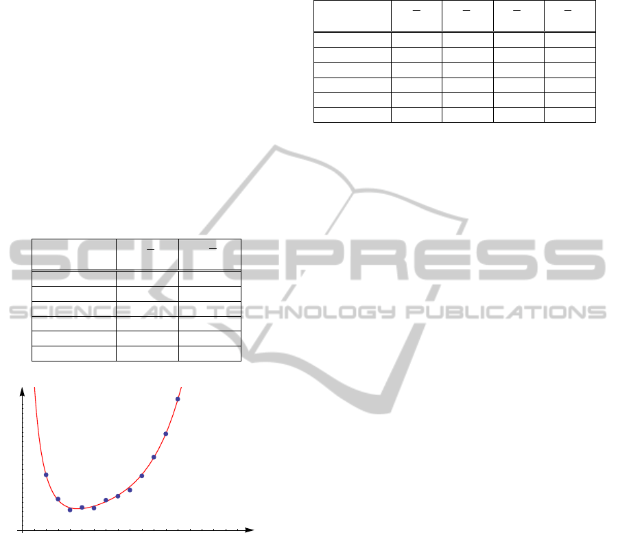
5.2.1 Simple Stunted Random Walk
We perform 50000 runs of simulation using simple
stunted random walk strategies. We found the results
are similar to the ones using exact method using
Markov chain theory (see Table 3). We also show
the comparison between the two results for the case
of initial random placement,
(, ),Trp on the graph in
Figure 2. This graphs shows that our simulation
provides outcomes which closely approximate the
ones calculated using the exact method.
Table 3: Simulation results of optimal expected times,
simple stunted random walk on L
3
(50000 runs).
Starting state
T
p
Random, r 4.1950 0.2350
s
1 =
[3,0,0] 6.2000 0.2300
s
2 =
[2,1,0] 3.9760 0.0600
s
3 =
[2,0,1] 5.3110 0.4900
s
4 =
[1,2,0] 2.9810 0.0400
s
5 =
[0,3,0] 5.2220 0.3100
Figure 2: Comparison of the expected times between the
two methods (exact method and simulation) for the case of
random initial placement T(r,p).
5.2.2 Compound Stunted Random Walk
From Table 4 below, we can see that the simulation
also gives results similar to the exact method shown
in Table 2. In particular, simulation can handle both
absorbing and non-absorbing chain in the same way,
unlike in the exact method where we need to
differentiate the approach between the two classes of
Markov chain.
Table 4: Simulation results of optimal expected times,
compound stunted random walk on L
3
(10000 runs).
Starting
state
T
1
p
2
p
3
p
Random, r 3.3115 1.0000 0.4900 0.1200
s
1 =
[3,0,0] 5.3159 0.9900 0.4900 0.1000
s
2 =
[2,1,0] 3.9385 0.0000 0.0400 0.6100
s
3 =
[2,0,1] 2.7392 0.9900 0.5400 0.0600
s
4 =
[1,2,0] 2.9532 0.0000 0.0000 0.0600
s
5 =
[0,3,0] 4.2666 0.9900 0.4700 0.1600
6 EXPECTED OUTCOME –
FURTHER RESEARCH
There are several directions of further research to be
carried out. The most obvious is to continue the
investigation to larger line graphs, such as
4
,L
5
,L
and eventually the class of
n
L in general. We also
plan to study other classes of graphs, in particular
the class
n
K
of complete graphs and the class
n
C of
cycle graphs. As both are transitive, all initial
placements of agents at a single node are equivalent,
which will simplify the analysis.
A second direction of research is to analyse how
strategies work on unknown graphs (mazes) or
random graphs. When sending in robots to search a
large house whose interconnecting room structure is
unknown, what is a good stationary probability p to
program them with?
Another possibility is the manager of the agents
observes the state and then broadcasts a ‘state-
dependent’ value of
p
or of the vector
.p
Finally, we could give our agents some limited
eyesight, so for example they might know the
current population of all nodes adjacent to their own.
The walk they choose in this case need not be
random, as neighboring nodes are distinguished by
their populations. Presumably one would go more
likely to a less populated node.
REFERENCES
Alpern, S., Gal, S., 2003. The theory of search games and
rendezvous. Kluwer Academic Publishers, Boston.
Alpern, S., Reyniers, D., 2002. Spatial Dispersion as a
Dynamic Coordination Problem. Theory Decis. 53,
29–59.
Arthur, W. B., 1994. Inductive Reasoning and Bounded
Rationality. Am. Econ. Rev. 84, 406–411.
Azar, Y., Broder, A., Karlin, A., Upfal, E., 1999. Balanced
Allocations. SIAM J. Comput. 29, 180–200.
0.2 0.4 0.6 0.8
p
4.2
4.4
4.6
4.8
5.0
5.2
T
r,
p
ANetworkDispersionProblemforNon-communicatingAgents
71

Challet, D., Zhang, Y.-C., 1997. Emergence of
cooperation and organization in an evolutionary game.
Phys. A Stat. Mech. its Appl. 246, 407–418.
Fretwell, S. D., Lucas Jr., H. L., 1969. On territorial
behavior and other factors influencing habitat
distribution in birds. Acta Biotheor. 19, 16–36.
Galceran, E., Carreras, M., 2013. A survey on coverage
path planning for robotics. Rob. Auton. Syst. 61, 1258–
1276.
Grenager, T., Powers, R., Shoham, Y., 2002. Dispersion
games: general definitions and some specific learning
results, in: AAAI-02 Proceedings. pp. 398–403.
Grinstead, C. M., Snell, J.L., 1997. Introduction to
Probability, 2nd ed., 2nd rev. e. ed. American
Mathematical Society.
Houston, A., McNamara, J., 1997. Patch choice and
population size. Evol. Ecol. 11, 703–722.
Qiu, L., Yang, Y. R., Zhang, Y., Shenker, S., 2003. On
Selfish Routing in Internet-like Environments, in:
Proceedings of the 2003 Conference on Applications,
Technologies, Architectures, and Protocols for
Computer Communications. ACM, New York, NY,
USA, pp. 151–162.
Rosenthal, R. W., 1973. A class of games possessing pure-
strategy Nash equilibria. Int. J. Game Theory 2, 65–
67.
ICAART2014-DoctoralConsortium
72
