
Economical Aspects of Database Sharding
Uwe Hohenstein
1
and Michael C. Jaeger
2
1
Siemens AG, Corporate Technology, CT RTC ITP SYI-DE, Otto-Hahn-Ring 6, D-81730 Muenchen, Germany
2
Siemens AG, Corporate Technology, CT CSG SWI OSS, Otto-Hahn-Ring 6, D-81730 Muenchen, Germany
Keywords: Public Cloud, Database Sharding, Economical Aspects, Scale Out, NoSQL.
Abstract: Database sharding is a technique to handle large data volumes efficiently by spreading data over a large
number of machines. Sharding techniques are not only integral parts of NoSQL products, but also relevant
for relational database servers if applications prefer standard relational database technology and also have to
scale out with massive data. Sharding of relational databases is especially useful in a public cloud because
of the pay-per-use model, which already includes licenses, and the fast provisioning of virtually unlimited
servers. In this paper, we investigate relational database sharding thereby focussing in detail on one of the
important aspects of cloud computing: the economical aspects. We discuss the difficulties of cost savings
for database sharding and present some surprising findings on how to reduce costs.
1 INTRODUCTION
Recently, a new storage technology named NoSQL
has come up (NoSQL, 2013). The NoSQL idea takes
benefit, among others, from placing data on several
nodes, being able to store massive data just by
adding nodes and thereby parallelizing operations.
However, there are applications in industrial
environments that want or have to retain standard
relational database systems (RDBSs) because of its
ad-hoc query capability and the query power of SQL
– both mostly missing in NoSQL – besides being a
well-established and mature technology.
In contrast to the scale out of NoSQL products,
RDBSs are designed to scale up by using bigger
machines, several disks and advanced concepts such
as table partitioning, frequently sticking to a single
RDBS server for query processing. However, there
is always a bleeding edge of what is possible so that
one cannot “go big” forever (Kharchenko, 2012).
Database sharding for larger data volumes is one
solution to scale out. The tables are sharded, i.e., are
split by row and spread across multiple database
servers, the shard members or partitions, according
to a distribution key. The distribution key specifies a
range value for each shard member. The main
advantage of database sharding is the ability to grow
in a linear fashion as more servers are included to
the system. Another positive effect is that each
database shard can be placed on separate hardware
thus enabling a distribution of the database over a
large number of machines, resulting in less
competition on resources such as CPU, memory, and
disk I/O. This means that the database performance
can be spread out over multiple machines taking
benefit from high parallelism. Since the number of
rows in each table in each database is also reduced,
performance is improved by having smaller search
spaces and reduced index sizes. In addition, if the
partitioning scheme is based on some appropriate
real-world segmentation of the data, then it may be
possible to infer and to query only the relevant
shard. Moreover, there will be an increase of
availability since data is distributed over shards: If
one shard fails, other shards are still available and
accessible. And finally, (Kharchenko, 2012) shows
that sharding can save costs compared to scaling up.
RDBSs, and particularly RDBS sharding, make
also sense for cloud applications. In fact, RDBS
products are available in public cloud PaaS
offerings: Microsoft Azure SQL Database (SQL
Server in the Microsoft Cloud), Amazon RDS
(supporting MySQL, Oracle, Microsoft SQL Server,
or PostgreSQL systems), or offerings from IBM,
Oracle, and others. These products are similar to on-
premises servers, however, managed by the cloud
provider. This reduces administrative work for users.
RDBSs as well as other resources can be pro-
visioned in short time, and resources are principally
virtually unlimited (Armbrust, 2010). Due to a pay-
417
Hohenstein U. and C. Jaeger M..
Economical Aspects of Database Sharding.
DOI: 10.5220/0004944604170424
In Proceedings of the 4th International Conference on Cloud Computing and Services Science (CLOSER-2014), pages 417-424
ISBN: 978-989-758-019-2
Copyright
c
2014 SCITEPRESS (Science and Technology Publications, Lda.)

as-you-go principle, users have to pay only for those
resources they are actively using, on a timely basis.
Hence, it is easy to rent several RDBS instances in
order to scale out and to overcome size limitations.
There is also no need to take care of licenses since
they are already part of the PaaS offerings and
captured by the cost model. However, some
limitations such as a 150GB limit for Azure SQL
databases and a couple of functional restrictions with
regard to on-premises products have to be taken into
account.
The idea of database sharding is principally well
investigated, for instance, elaborating on sharding
strategies (Obasanjo, 2009) or discussing challenges
such as load balancing (Louis-Rodríguez, 2013) and
scaling (Kharchenko, 2012). A lot of work tries to
compare distributed relational databases with
NoSQL (Cattell, 2011). Anyway, comparisons
between RDBSs and NoSQL sometimes appear as
ideological discussions rather than technical
argumentations, as pointed out by (Kavis, 2010)
(Moran, 2010). Sharding is also partially supported
by cloud providers. In the Azure federation
approach, for instance, special operations are
available to split and merge shards in a dynamic
manner with no downtime; client applications can
continue accessing data during repartitioning
operations with no interruption in service.
In this paper, we tackle an important industrial
aspect: the operational costs of database sharding in
the cloud. In general, existing work on economical
aspects of cloud computing is very few (cf. Section
2). Most publications and white papers rather relate
to a Total Cost of Ownership (TCO) comparison
between on premise and cloud deployments. But
there is only little work such as (Hohenstein, 2012)
on reducing costs in the cloud – if the decision for
the cloud has been taken. Hence, we focus on cost
aspects of database sharding in the cloud in detail.
The remainder of this paper is structured as
follows. Section 2 provides an overview of related
work and detects the lack of research. Afterwards,
cost considerations for a simple, but common
pricing model are made in Section 3. In particular,
we discuss the difficulties of how to reduce storage
costs by sizing and splitting partitions appropriately.
Section 4 tackles another aspect of sharding that
must not be neglected – performance issues. Indeed,
cost and performance must be balanced. Further
architectural challenges of database sharding are
presented in Section 5 work before Section 6
concludes and discusses some future work.
2 RELATED WORK
Although (Armbrust, 2010) identifies short-term
billing as one of the novel features of cloud
computing and (Khajeh-Hosseini, 2010) considers
costs as one important research challenge for cloud
computing, only a few researchers have investigated
the economic issues around cloud computing from a
consumer and provider perspective. Even the best
practices of cloud vendors, for instance, (Microsoft,
2013) and (Kharchenko, 2012), do not particularly
indicate how to reduce costs.
Most work focuses on cost comparisons between
cloud and on-premises and lease-or-buy decisions.
(Walker, 2009) compares the costs of a CPU hour
when it is purchased as part of a server cluster, with
when it is leased for two scenarios. It turned out that
buying is cheaper than leasing when CPU utilization
is very high (over 90%) and electricity is cheap. To
widen the space, further costs such as housing the
infrastructure, installation and maintenance, staff,
storage and networking must be taken into account.
(Klems, 2009) provides a framework that can be
used to compare the costs of using a cloud with an
in-house IT infrastructure. Klems also discusses
some economic and technical issues that need to be
considered when deciding whether deploying
systems in a cloud makes economic sense.
(Assuncao, 2009) concentrates on a scenario of
using a cloud to extend the capacity of locally
maintained computers when their in-house resources
are over-utilized. They simulated the costs of using
various strategies when borrowing resources from a
cloud provider, and evaluated the benefits by using
the Average Weighted Response Time (AWRT)
metrics (Grimme, 2008).
(Kondo, 2009) examines the performance trade-
offs and monetary cost benefits of Amazon AWS for
volunteered computing applications of different size
and storage.
(Palankar, 2008) uses the Amazon data storage
service S3 for scientific intensive applications. The
conclusion is that monetary costs are high because
the service covers scalability, durability, and
performance – services to be paid but often not
required by data-intensive applications. In addition,
(Garfinkel, 2007) conducts a general cost-benefit
analysis of clouds without any specific application.
(Deelman, 2008) highlights the potentials of
using cloud computing as a cost-effective deploy-
ment option for data-intensive scientific applica-
tions. They simulate an astronomic application and
run it on Amazon AWS to investigate the
performance-cost tradeoffs of different internal
CLOSER2014-4thInternationalConferenceonCloudComputingandServicesScience
418

execution plans by measuring execution times,
amounts of data transferred to and from AWS, and
the amount of storage used. They found the cost of
running instances to be the dominant figure in the
total cost of running their application. Another study
on Montage (Berriman, 2010) concludes that the
high costs of data storage, data transfer and I/O in
case of an I/O bound application like Montage
makes AWS much less attractive than a local
service.
(Kossmann, 2010) performs the TPC-W
benchmark for a Web application with a backend
database and compares the costs for operating the
web application on major cloud providers, using
existing relational cloud databases or building a
database on top of table or blob storages.
(Hohenstein, 2012) showcases with concrete
examples how architectures impact the operational
costs, once the decision to work in the cloud has
been taken. Various architectures using different
components such as queues and table storage are
compared for two scenarios implemented with the
Windows Azure platform. The results show that the
costs can vary dramatically depending on the
architecture and the applied components.
Concerning sharding, (Biyikoglu, 2011) tackles
the question “how do you cost optimize
federations?” for Azure SQL federations. The paper
recommends consolidating storage to fewer
members for cost conscious systems, thus saving on
cost but risk higher latency for queries. For mission
critical workloads, more money should be invested
in order to spread too many smaller members for
better parallelism and performance. Since every
application’s workload characteristics are different,
there is no declared balance-point. Thus, Biyikoglu
recommends testing the workload and measure the
query performance and cost under various setups.
To our knowledge, trying to reduce costs within
a certain cloud is not well investigated. We tackle
this deficit by optimizing database sharding cost.
3 COST CONSIDERATIONS
This paper is mainly concerned with an economical
perspective of database sharding in the cloud since
costs are relevant for industrial applications. In fact,
pay-as-you-go is one important characteristic of
cloud computing (Armbrust, 2010). As (Hohenstein,
2012) pointed out, there is a strong need for cost
saving strategies in a public cloud. One important
question we are investigating in this context is: how
to size shards for achieving optimal costs?
3.1 A Sample Pricing Model
The pricing models of public cloud providers are
mainly based upon certain factors such as storage,
data transfer in and out etc. Most have in common
that the more resources one occupies or consumes,
the less expensive each resource becomes.
In the following, we use the pricing model of a
popular public cloud provider. We keep the name
anonymous because we do not want to promote one
specific provider. Anyway, our main statements can
be transferred to other providers analogously even if
the price models and the relevant factors differ. Our
main intention is to illustrate the challenges with
pricing models in the public cloud.
In the pricing model, each database in use has to
be paid depending on the storage consumption, i.e.,
the size of the database:
0 to 100 MB: $4.995 (fix price)
100 MB to 1 GB: $9.99 (fix price)
1 GB to 10 GB: $9.99 for the first GB,
$3.996 for each additional GB
10 GB to 50 GB: $45.96 for the first 10 GB,
$1.996 for each additional GB
50 GB to 150 GB: $125.88 for the first 50 GB,
$0.999 for each additional GB
Hence, a 20GB is charged with $65.92; $45.96 for
the first 10GB and 10*$1.996 for the next 10GB.
Similarly, an 80GB database costs $155.85 ($125.88
for the first 50GB and 30*0.999 for the next 30GB),
while 150GB sum up to $225.78. These prices are
on a monthly basis. The maximal amount of data is
measured every day, and each day is charged
according to the monthly fee. Hence, Using 10GB
for the first ten days and 60 GB for the next 5 days is
charged with $37.96 ($45.96*10/30 + $135.87*5/30)
for 15 days. Also note that pricing occurs in incre-
ments of 1GB. Hence, 1.1GB is charged as 2GB.
3.2 Simple Considerations
In case of database sharding, each database shard is
charged that way. Unfortunately, reducing costs for
sharding is not that simple as it seems to be.
We start with some simple considerations for the
above pricing model. Let us first compare ten 10GB
databases (a) with one 100GB database (b). Both are
able to store 100GB, but the prices differ a lot:
a) 10 * 10GB à $45.96 each = $459.60
b) 1 * 100GB = $175.83
That is, one large partition is 3.8 times cheaper in a
month than 10 smaller ones making up a difference
EconomicalAspectsofDatabaseSharding
419
of $284. The monthly difference is even larger in the
following case of storing 1,200GB:
a) 120 * 10GB = 120 * $45.96 = $5,515.20
b) 8 * 150GB = 8 * $225.78 = $1,806.24
Here, the factor is about 3 or absolutely $3,700 a
month! These examples show clearly that it is more
economic to use a few databases of larger sizes than
more small-size databases.
Unfortunately, smaller databases provide a better
query performance the effect of which is even
stronger in the cloud since databases reside on
different servers having their own resources. Both
setups have access to the same storage capacity,
however clearly 120x10GB databases have access to
15 times more cores, memory and IOPS capacity as
well as temporary space and log files. Thus, the
costs must be balanced with performance
requirements to be achieved.
Let us assume that performance measurements
detect that 100GB is a reasonable partition size
regarding given performance requirements.
The previous analysis referred to a rather static
view. For dynamic data, the question arises how to
split a partition if the 100GB limit is exceeded. The
most intuitive split will certainly be balanced with
50/50%. But is this really the best choice?
a) 50 + 50 GB: 2 * $125.88 = $251.76
b) 80 + 20 GB: $155.85 + $65.92 = $221.77
The split into 80 and 20 GB (b) is $30 cheaper, with
the effect that the first partition will again flow over
after 20 additional GB: this is not really a cost
problem but the performance might be affected by
too many splits and unbalanced partitions.
If we now add further 30GB to both partitions in
this scenario, we obtain the following costs: In case
of (a), 15 GB are put into both partitions equally:
a) 65GB + 65GB: 2 * $140.865 = $281.73
In case of (b), we add 24GB to the first and 6GB to
the second partition, assuming an equal distribution
of the new 30GB according to the previous split
ratio 80/20%. This means another split becomes
necessary for the 80+24=104GB database resulting
in 83,2GB and 20,8GB partitions. Now, (b) turns out
to be $24 more expensive:
b) $159.846 (83.2GB + $67.916 (20.8GB)
+ $77.896 (26GB) = $305.658
3.3 Long-term Comparison
Obviously, it is necessary to calculate the cumulated
costs over a longer period of time. As a more
elaborated example, we start with 100GB (exactly
the partition limit), and assume a daily increase of 1
GB, equally distributed over the partition key.
Table 1 summarizes the database sizes and the
costs for the first 50 days for a 50/50% split ratio.
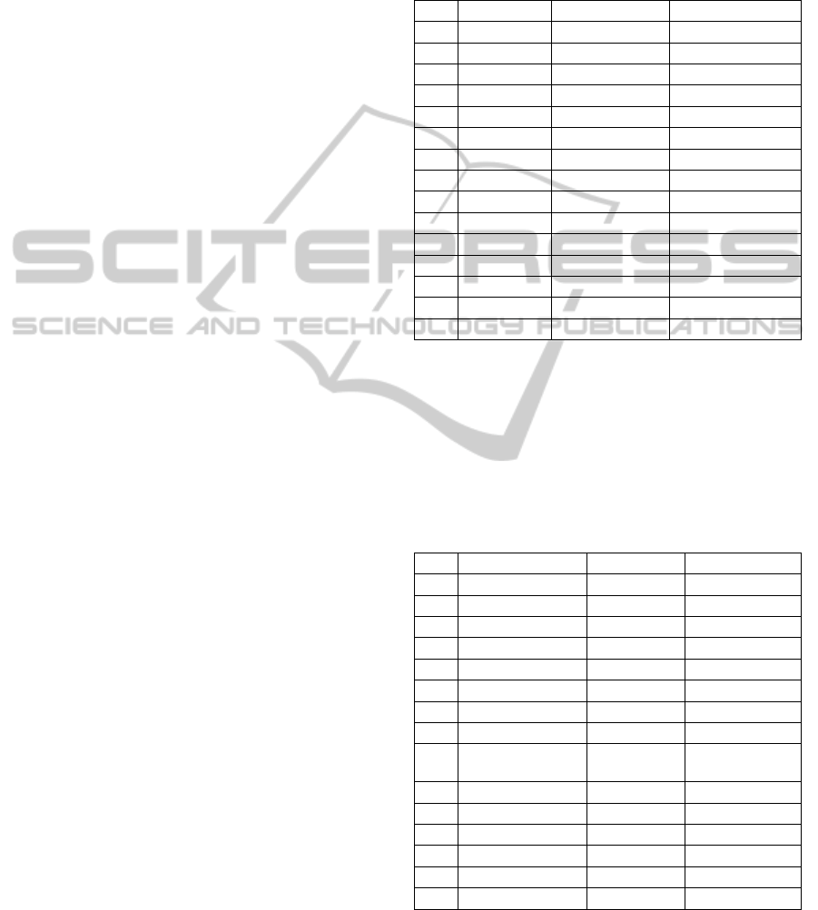
Table 1: Costs for 50/50% ratio.
day databases costs for day x cumulated costs
1 2 * 50.5 $253.758 / 30 $8.45
2 2 * 51 $253.758 / 30 $16.91
…
10 2 * 55 $261.750 / 30 $85.91
…
20 2 * 60 $271.740 / 30 $175.16
…
25 2 * 62.5 $277.7340 / 30 $221.05
26 2 * 63 $277.7340 / 30 $230.31
…
30 2 * 65 $281.730 / 30 $267.74
…
40 2 * 70 $291.720 / 30 $363.65
…
50 2 * 75 $301.710 / 30 $462.89
Please note that the costs for the “price for day
x” column should be divided by 30 (“/ 30”) in order
to obtain the daily costs. The cumulated costs sum
up the daily costs until day x. Keep also in mind that
database sizes are rounded up to full GBs, i.e.,
50.5GB are taken as 51GB and charged with
$253.758 per month.
Table 2: Costs for 80/20% ratio.
day databases costs for day x cumulated costs
1 80.8 + 20.2 $224.765 / 30 $7.49
2 81.6 + 20.4 $225.764 / 30 $15.01
…
10 88 + 22 $233.754 / 30 $76.51
…
20 96 + 24 $245.738 / 30 $157.03
…
25 100 + 25 $251.73 / 30 $198.78
26 80.64 + 20.16
(split!) + 25.2
$302.661 / 30 $208.87
…
30 83.20 + 20.80 + 26 $305.658 / 30 $249.46
…
40 89.60 + 22.40 + 28 $319.636 / 30 $354.21
…
50 96.00 + 24.00 + 30 $331.618 / 30 $463.42
Table 2 summarizes the database sizes and the
costs for the first 50 days for an 80/20% ratio, being
applied recursively: Each partition is again split with
CLOSER2014-4thInternationalConferenceonCloudComputingandServicesScience
420
this ratio. The total costs are lower for the 80/20%
ratio during the first days: There is a benefit of $0.96
for the first day, $18.13 for the first 20 days, and
$18.28 for the first 30 days. But we notice a change
at day 50: the 50/50% ratio becomes cheaper.
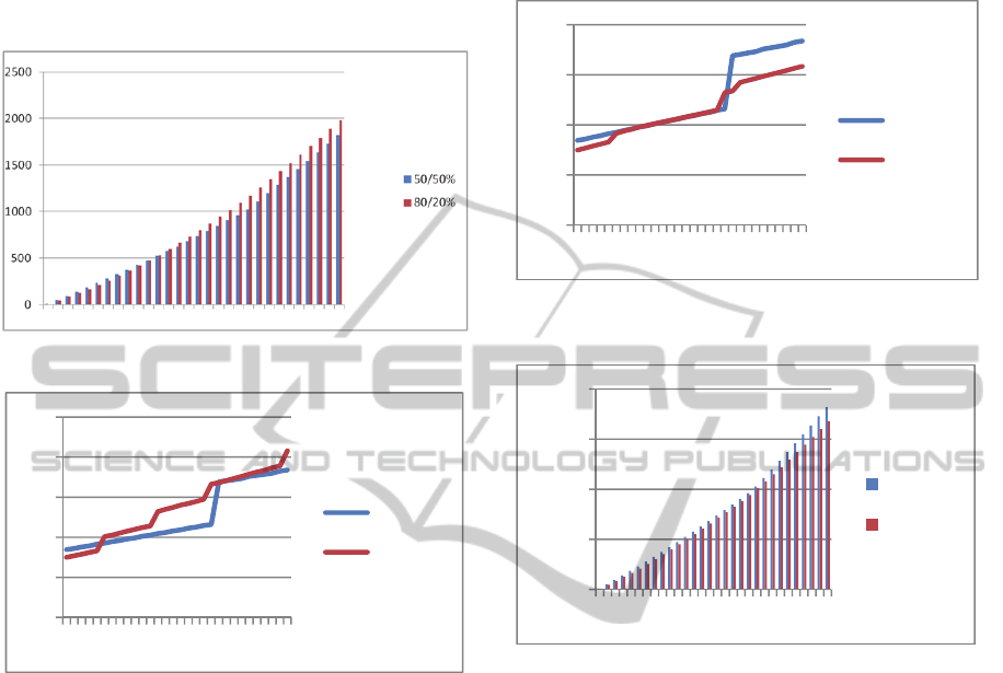
Figure 1: Long-term comparison of cumulated costs.
Figure 2: Long-term comparison of daily prices.
Figure 1 compares the total costs for the first 150
days. It shows that 50/50% becomes cheaper and
stays cheaper after 50 days; the difference is even
increasing day by day.
As Figure 2 shows, the reason is that the price
for each day increase a lot from day 25 to 26 (cf.
also Table 1 and 2). After 26 days, the daily price of
the 50/50% ratio becomes cheaper for each
successive day; after day 56, the gap gets even larger
due to an additional increase at that day.
If we dive into the details, we notice that the
number of smaller partitions has increased at those
days. In fact, a split occurs at day 26 for the 80/20%
ratio: A partition with 100.8GB is split into 80.64GB
and 20.16GB. This means three partitions of
80.64GB, 20.16GB, and 25.2GB occur at day 26,
with a daily price of $302.661 / 30 in contrast to
$251.73 / 30 the day before (cf. Table 2). This is an
increase of $1.69. We now pay $10.08 for that day
compared to $9.25 for the 50/50% ratio. Indeed, the
small partitions are dominating the costs, and at day
50 the total costs for 50/50% start to become
cheaper. Later on, further splits occur and affect the
comparison more negatively.
Figure 3: Long-term comparison of cumulated costs (with
merge strategy).
Figure 4: Long-term comparison of daily prices (with
merge strategy).
3.4 Improvement
Anyway, there are alternatives to improve costs. The
basic idea to reduce costs is to get rid of smaller
partitions by means of merging them. In the previous
scenario, we can merge the two smaller partitions of
20.16GB and 25.2GB at day 26 right after the split:
partitions with 20.16GB and 25.2GB: $145.812
one merged partition with 45.36GB: $117.816
Thus, merging partitions reduces the costs at day 26
by $27.996/30 = 93ct. Using this merge strategy for
the evaluation, we can improve the daily price
dramatically (cf. Figure 3). The costs for 80/20%
remain below 50/50% with a few exceptions. This
leads to the cost comparison in Figure 4. Using the
80/20% ratio becomes always cheaper and the
savings to 50/50% increases day by day. Now, we
benefit from the 80%/20% ratio even in the long run.
We conclude this section with demonstrating
what monetary benefit can be achieved by choosing
the best ratio compared to a 50/50% split:
0
5
10
15
20
25
50/50%
80/20%
0
5
10
15
20
50/50%
80/20%
0
500
1000
1500
2000
50/50%
80/20%
50 100 150
50 100 150
50 100 150
50 100 150
EconomicalAspectsofDatabaseSharding
421

$13.98 savings for 100 days
$1239.48 savings for 500 days
$5090.39 savings for 1000 days
One important issue remains open: What is the
optimal split ratio? We implemented an algorithm to
find out optimal ratios for scenarios given by initial
size, daily increase, and number of days. It turned
out that a ratio between 0.8 and 0.9 will be most
cost-efficient for 100GB shards and 1GB increm-
ents. The optimal ratio varies from day to day, but it
mostly stays in this interval. Even if the split ratio
does not strike the optimum, costs can be reduced
compared to a 50/50% split.
Other partition sizes and/or increments certainly
lead to other results. But most of our tested scenarios
do not let the 50/50% ratio be the best solution.
In principal, it is necessary to make an analytical
investigation for finding a formula and making a lim
1→∞ calculation; this is subject to future research.
4 PERFORMANCE
Saving costs is certainly one important driver in
industrial use cases. Anyway, the cost reduction
must also be seen in the context of performance.
Performance requirements will affect the size of
partitions. Thus, this section presents some basic
performance results. We essentially compare using
ten (smaller) 1GB databases with using one (larger)
10GB database.
4.1 Test Setup for Ten 1GB Databases
We use the following table structure for each of the
shard members:
ShardedTable(k int, id int,
t10 int, t100 int, tf500 float, v100
varchar(100), v200 varchar(200), v300
varchar(300), doc xml)
.
Each of the 10 shard members contains
1,000,000 records, summing up to 10GB including
indexes for all 10 shards. Column
k is the primary
key, which is globally unique over all partitions.
Each partition has different ranges of keys, i.e., the
first partition k=0..999,999, the second one with
k=1,000,000..1,999,999, and so on. In contrast,
id is
a successive number that is only locally unique
within each shard. Column
doc contains an XML
document representing the complete record as XML.
We implemented a REST service that executes
arbitrary queries with parameterized values. The
REST service runs in a VM of its own in a public
cloud, in the same data centre as the database shards.
The service URL has the following structure:
http://<MyServer>/QueryService/query
?txt=<query>¶m=@k&value=80000
We can perform a parameterized <query> such
as
SELECT * FROM ShardedTable WHERE k=@k
from any Web browser; value for parameter
@k is
here 80000. There is an optional request parameter
db that allows for specifying a single database (as in
case of the 10 GB database). Without, a thread pool
is spanned for executing the same query on all
shards in parallel. We certainly measure only the
execution time within the REST server, i.e., without
the latency to the query service. The execution times
are returned as part of the REST response.
4.2 Test Setup for One 10GB Database
To keep the same data volume as in 4.1, the 10GB
database is set up with 10,000,000 records enume-
rated from 0 to 9,999,999. The table structure is the
same as before, however,
k is the primary key for all
the records while each
id value refers to 10 records.
4.3 Test Scenarios
We investigated and compared the performance of
three scenarios:
a) Access to all ten 1GB shards in parallel
b) Access to one 10GB database
c) Access to one single 1GB shard
The last scenario is relevant if the shard to be
queried is known; then no parallel query has to be
executed.
The measurements are taken ten times each at
different times of a day. This explains the broader
variance in the results.
We first present the very first execution times of
requests, i.e., no caching will take place. Table 3
summarizes the results for searching a primary key
value (column
k). In any case, the result will be a
single record, i.e., the record will be found in one of
the shards. As expected, searching a single shard (if
the partition is known) is performing best. But it is
surprising that an (index-based) search in 10GB is
faster than parallelizing ten requests to 1GB shards
and combining the results.
Table 4 presents the execution times for
accessing records with a given
id value. The id
column is not indexed! In case of sharding, each of
the ten shards returns a single record; the 10GB
database returns 10 records analogously. Now,
sharding produces 4 times better results than a 10GB
database. Again, searching one record in a single
1GB database is outstanding, but irrelevant since
CLOSER2014-4thInternationalConferenceonCloudComputingandServicesScience
422
each shard contributes to the overall result.
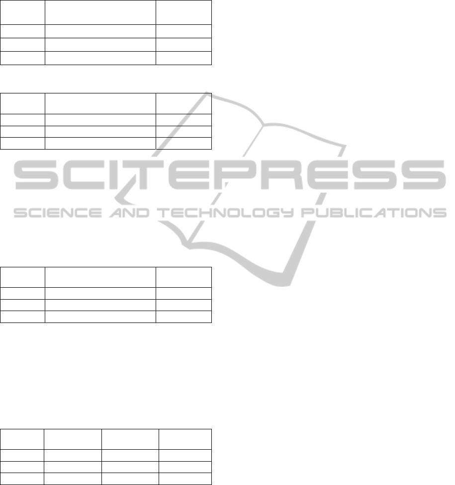
Table 3: Global key search.
Scenario Average elapsed time [ms] Standard
deviation
10 * 1GB 622.9915 241.6767746
1 * 10GB 437.4642 786.1302572
1 * 1GB 166.0001 255.7591507
Table 4: Full table scan.
Scenario Average elapsed time [ms] Standard
deviation
10 * 1GB 5950.63548 2402.86658
1 * 10GB 22161.99186 6534.50578
1 * 1GB 1050.68536 708.21466
Table 5 presents the results for searching an
indexed value (column t10) in all partitions. Each
sharded query returns 10 records, i.e., 100 in total;
the 10GB database returns 100 records as well. It is
again surprising, that the 10GB database beats the
sharded query. Even the difference to a single 1GB
query is small.
Table 5: Index-based search.
Scenario Average elapsed time [ms] Standard
deviation
10 * 1GB 558.54096 684.1157257
1 * 10GB 189.43505 82.4324732
1 * 1GB 107.41177 64.3837701
To complete the analysis, we measured the
average execution times for each query, being
executed 5 times successively and excluding the
very first execution. Table 6 summarizes the results
for those “hot” queries, essentially confirming the
previous results.
Table 6: Successive accesses (in ms).
Scenario Global Key
Search
Full Table
Scan
Index-based
Search
10 * 1GB 50.2883937 1859.204 68.542061
1 * 10GB 16.6000000 5691.369 30.169731
1 * 1GB 12.2059406 671.324 8.788243
Thus, sharded queries might be expensive due to
the overhead of multithreading and consolidating
results. This means that partitions might be chosen
larger than expected in order to save costs. However,
we do not want to conclude here that using parallel
queries are less performing in general. Of course,
there are further aspects such as the size of the VM
to run the sharding layer, the thread pool, the PaaS
offering, means for co-location etc. Rather we want
to encourage developers to perform performance
tests by their own. As we stated in (Hohenstein,
1997), it is absolutely recommended to perform
application-specific benchmarks for meaningful
results taking into account the applications’
characteristics. Here, we simply wanted to get a first
impression about the performance behaviour.
5 FURTHER CHALLENGES
From an architectural point o view, it is a good idea
to introduce a sharding layer the purpose of which is
to distribute queries over member shards and to
consolidate responses. There are a couple of further
issues we want to mention briefly.
The sharding layer has to take care of connection
handling. In fact, each database has a connection
string of its own, which usually means that each
shard obtains a pool of its own. Thus, the sharded
connections are often not pooled in a shared pool.
There is a need for a shared meta database
directory that contains all configuration information,
in particular, about the physical shards, their
connection string etc.
The distribution scheme is important. If it is not
well-designed for the major use cases, then global
transactions and distributed joins across shards
cannot be avoided and the sharding layer has to take
care. Similarly, cross-shard sorting and aggregation
is another challenge for results from different shards.
Another important issue is certainly schema
evolution, i.e., changes to the table structures. Any
schema upgrade must be rolled out to all members.
Rebalancing of shards (removing and adding
shards) is a performance issue. Usually, databases
have to be created or deleted and data has to be
moved between databases.
Finally, we want to mention certain technical
issues such as policies for key generation, shard
selection, construction of queries and operations.
6 CONCLUSIONS
Sharding of RDBSs is relevant if applications have
to stick to relational database technology, but
scalability or Big Data issues arise at the same time.
Sharding enables one to add additional database
servers to handle growing data volumes and to
increase scalability. This is particularly of interest
for cloud computing environments because of the
pay-as-you-go principle and the ease to provision
EconomicalAspectsofDatabaseSharding
423

new database servers in short time.
In this paper, we investigated database sharding
of relational database systems (RDBS) in the cloud
from the perspective of cost and performance. We
obtained some surprising results.
At first, splitting shards into two equally sized
shards is not always advantageous from a cost
perspective. Other split factors such as 80/20%,
combined with a merge operation, yield better
results in our scenarios. Anyway, we demonstrated
that achieving optimal costs is difficult in general.
Furthermore, performance measurements show
that parallelizing queries to several shards is not
always better than querying a single database of the
same total size.
In the future, we intend to further elaborate on
strategies to split optimally according to incoming
load. In particular, cost/performance considerations
require further investigations. And finally, we want
to apply our ideas to multi-tenancy.
REFERENCES
Armbrust, M., Fox, A., Griffith, R., Joseph, A., Katz, R.,
Konwinski, A., Lee, G., Patterson, D., Rabkin, A.,
Stoica, I. and Zaharia, M. (2010): A View of Cloud
Computing. CACM, 53(4), April 2010.
Assuncao, M., Costanzo, A. and Buyya, R. (2009).
Evaluating the cost-benefit of using cloud computing
to extend the capacity of clusters. In HPDC '09: Proc.
of 18th ACM int. symposium on High performance
distributed computing, Munich, Germany, June 2009.
Berriman, B., Juve, G., Deelman, E., Regelson, M. and
Plavchan, P. (2010). The Application of Cloud
Computing to Astronomy: A Study of Cost and
Performance. 6th IEEE Int. Conf. on e-Science.
Biyikoglu, C. (2011): Pricing and Billing Model for
Federations in SQL Azure Explained! http://
blogs.msdn.com/b/cbiyikoglu/archive/2011/12/12/billi
ng-model-for-federations-in-sql-azure-explained.aspx
Cattell, R. (2011): Scalable SQL and NoSQL Data Stores.
ACM SIGMOD Record, Vol. 39(4).
Deelman, E., Singh, G., Livny, M., Berriman, B. and
Good, J. (2008). The cost of doing science on the
cloud: the Montage example. In Proc. of 2008 ACM/
IEEE conf. on Supercomputing, Oregon, USA, 2008.
Garfinkel, S. (2007). Commodity Grid Computing with
Amazon S3 and EC2. In login 2007.
Greenberg, A., Hamilton, J., Maltz, D. and Patel, P.
(2009). The Cost of a Cloud: Research Problems in
Data Center Networks. ACM SIGCOMM Computer
Communication Review, 39, 1.
Grimme, C., Lepping, J. and Papaspyrou, A. (2008).
Prospects of Collaboration between Compute
Providers by means of Job Interchange. In Proc. of
13th Job Scheduling Strategies for Parallel
Processing, April 2008, LNCS 4942.
Hamdaqa, M., Liviogiannis, L. and Tavildari, L. (2011): A
Reference Model for Developing Cloud Applications.
Int. Conf. on Cloud Computing and Service Science
(CLOSER) 2011.
Hohenstein, U., Krummenacher, R., Mittermeier, L. and
Dippl, S. (2012): Choosing the Right Cloud
Architecture - A Cost Perspective. CLOSER’2012.
Hohenstein, U., Plesser, V., Heller, R. (1997): Evaluating
the Performance of Object-Oriented Database Systems
by Means of a Concrete Application. DEXA 1997.
Kavis, M. (2010): NoSQL vs. RDBMS: Apples and
Oranges. http://www.kavistechnology.com/blog
/nosql-vs-rdbms-apples-and-oranges.
Khajeh-Hosseini, A., Sommerville, I. and Sriram, I.
(2011). Research Challenges for Enterprise Cloud
Computing. 1st ACM Symposium on Cloud
Computing, SOCC 2010, Indianapolis.
Kharchenko, M. (2012): The Art of Database Sharding.
http://intermediatesql.com/wp-content/uploads/2012
/04 /2012_369_Kharchenko_ppr.doc
Klems, M., Nimis, J. and Tai, S. (2009). Do Clouds
Compute? A Framework for Estimating the Value of
Cloud Computing. Designing E-Business Systems.
Markets, Services, and Networks, Lecture Notes in
Business Information Processing, 22.
Kondo, D., Javadi, B., Malecot, P., Cappello, F. and
Anderson, D. P. (2009). Cost-Benefit Analysis of
Cloud Computing versus Desktop Grids. In Proc. of
the 2009 IEEE Int. Symp. on Parallel&Distributed
Processing, May 2009.
Kossmann, D., Kraska, T. and Loesing, S. (2010). An
Evaluation of Alternative Architectures for Trans-
action Processing in the Cloud. ACM SIGMOD 2010
Louis-Rodríguez, M., Navarro, J., Arrieta-Salinas, I.,
Azqueta-Alzuaz, A. Sancho-Asensio, A. and
Armendáriz-Iñigo, J. E.: Workload Management for
Dynamic Partitioning Schemes in Replicated
Databases. CLOSER’2013.
Moran, B. (2010): RDBMS vs. NoSQL: And the Winner
is… http://sqlmag.com/sql-server/rdbms-vs-nosql-and-
winner.
Microsoft (2013): Windows Azure .Net Developer Center -
Best Practices. http://www.windowsazure.com/en-
us/develop/net/best-practices.
NoSQL (2013): List of NoSQL Databases. http://nosql-
database.org
Obasanjo, D. (2009): Building Scalable Databases: Pros
and Cons of Various Database Sharding Schemes.
http://www.25hoursaday.com/weblog/2009/01/16
/BuildingScalableDatabasesProsAndConsOfVariousD
atabaseShardingSchemes.aspx.
Palankar, M., Iamnitchi, A., Ripeanu, M. and Garfinkel, S.
(2008). Amazon S3 for Science Grids: A Viable
Solution? In: Data-Aware Distributed Computing
Workship (DADC), 2008.
Walker, E. (2009). The Real Cost of a CPU Hour.
Computer, 42, 4.
CLOSER2014-4thInternationalConferenceonCloudComputingandServicesScience
424
