Graph Mining for Automatic Classiﬁcation of Logical Proofs

Karel Vacul

ık and Lubo

s Popel

ınsk

Knowledge Discovery Lab, Faculty of Informatics, Masaryk University, Botanick

a 68a,

CZ-602 00 Brno, Czech Republic

Keywords:

Graph Mining, Frequent Subgraphs, Logic Proofs, Resolution, Classiﬁcation, Educational Data Mining.

Abstract:

We introduce graph mining for evaluation of logical proofs constructed by undergraduate students in the intro-

ductory course of logic. We start with description of the source data and their transformation into GraphML.

As particular tasks may differ—students solve different tasks—we introduce a method for uniﬁcation of res-

olution steps that enables to generate generalized frequent subgraphs. We then introduce a new system for

graph mining that uses generalized frequent patterns as new attributes. We show that both overall accuracy

and precision for incorrect resolution proofs overcome 97%. We also discuss a use of emergent patterns and

three-class classiﬁcation (correct/incorrect/unrecognised).

1 INTRODUCTION

Resolution in propositional logic is a simple method

for building efﬁcient provers and is frequently taught

in university courses of logic. Although the struc-

ture of such proofs is quite simple, there is, up to

our knowledge, no tool for automatic evaluation of

student solutions. Main reason may lie in the fact

that building a proof is in essence a constructive task.

It means that not only the result—whether the set

of clauses is contradictory or not—but rather the se-

quence of resolution steps is important for evaluation

of correctness of a student solution.

If we aimed at error detection in a proof only, it

would be sufﬁcient to use some search method to ﬁnd

the erroneous resolution step. By this way we even

would be capable to detect an error of particular kind,

like resolution on two propositional letters. However,

there are several drawbacks of this approach. First,

detection of an error not necessary means that the so-

lution was completely incorrect. Second, and more

important, by search we can hardly discover patterns,

or sequence of patterns, that are typical for wrong

solutions. And third, for each kind of task – reso-

lution proofs, tableaux proofs etc. – we would need

to construct particular search queries. In opposite, the

method described in this paper is usable, and hope-

fully useful, without a principal modiﬁcation for any

logical proof method for which a proof can be ex-

pressed by a tree.

In this paper we propose a method that employs

graph mining (Cook and Holder, 2006) for classiﬁ-

cation of the proof as correct or incorrect. As the

tasks—resolution proofs—differs, there is a need for

uniﬁed description of this kind of proofs. For that

reason we introduce generalized resolution schemata,

so called generalized frequent subgraphs. Each sub-

graph of a resolution proof is then an instance of one

generalized frequent subgraph. In Section 2 we in-

troduce the source data and their transformation into

GraphML (GraphML team, 2007). Section 3 dis-

cusses preliminary experiments with various graph

mining algorithms. Based on these results, in Sec-

tion 4 we ﬁrst introduce a method for construction

of generalized resolution graphs. Then we describe

a system for graph mining that uses different kinds

of generalized subgraphs as new attributes. We show

that both overall accuracy and precision for incor-

rect resolution proofs overcome 97%. Discussion and

conclusion are in Sections 5 and 6, respectively.

2 DATA AND DATA

PRE-PROCESSING

The data set contained 393 different resolution proofs

for propositional calculus, 71 incorrect solutions and

322 correct ones. Each student solved and handwrote

one task. Two examples of solutions are shown in

Fig. 1.

To transform the students proofs into an electronic

version we used GraphML (GraphML team, 2007),

which uses an XML-based syntax and supports wide

range of graphs including directed, undirected, mixed

563

Vaculík K. and Popelínský L..

Graph Mining for Automatic Classiﬁcation of Logical Proofs.

DOI: 10.5220/0004963405630568

In Proceedings of the 6th International Conference on Computer Supported Education (CSEDU-2014), pages 563-568

ISBN: 978-989-758-020-8

 2014 SCITEPRESS (Science and Technology Publications, Lda.)

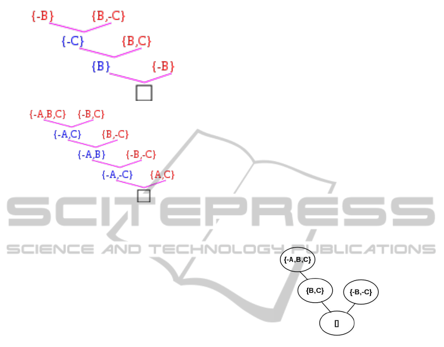
Figure 1: An example of a correct and an incorrect resolu-

tion proof.

graphs, hypergraphs, etc.

Common errors in proofs are the following: rep-

etition of the same literal in the clause, resolving on

two literals at the same time, incorrect resolution—

the literal is missing in the resolved clause, resolv-

ing on the same literals (not on one positive and one

negative), resolving within one clause, resolved lit-

eral is not removed, the clause is incorrectly copied,

switching the order of literals in the clause, proof is

not ﬁnished, resolving the clause and the negation of

the second one (instead of the positive clause).

3 FINDING CHARACTERISTIC

SUBGRAPH FOR RESOLUTION

PROOFS

The ﬁrst, preliminary, experiment—ﬁnding charac-

teristic subgraphs for incorrect and correct resolution

proofs—aimed at evaluating the capabilities of partic-

ular algorithms. They were performed on the whole

set of data and then separately on the sets representing

correct and incorrect proofs. The applications pro-

vided frequent subgraphs as their output for each set

of data which help in identifying and distinguishing

between subgraphs that are characteristic for correct

and incorrect proofs, respectively. One such subgraph

is depicted in Fig. 2.

Speciﬁcally, we performed several experiments

with four algorithms (Brauner, 2013)—gSpan (Yan

and Han, 2002), FFSM (Huan et al., 2003), Sub-

due (Ketkar et al., 2005), and SLEUTH (Zaki, 2005).

With gSpan we performed experiments for different

minimal relative frequencies ranging from 5 to 35 per

cent. The overall running time varied from a few mil-

liseconds to tens of milliseconds and the number of

resulting subgraphs for all three data sets varied from

hundreds to tens according to the frequency. Size

of the output varied from hundreds to tens of kilo-

bytes. With FFSM we tuned the parameters of our

experiments so that the results were comparable to

gSpan. Comparable numbers of resulting subgraphs

were obtained in less time with FFSM. Despite the

two-ﬁle output representation, the size of the output

was slightly smaller in comparison to gSpan. With

Subdue we performed several experiments for differ-

ent parameter settings. The results were promising:

we obtained from 60 to 80 interesting subgraphs in

less than tenths of a second. The maximal size of out-

put was 20 kilobytes. Unlike Subdue, SLEUTH ﬁnds

all frequent patterns for a given minimum support.

Figure 2: Characteristic subgraph for incorrect resolution

proofs.

To sum up the examined methods for mining in

general graphs, although all of them are acceptable

for our purpose, Subdue and SLEUTH seemed to be

the best. Subdue offers a suitable input format that is

convenient for data classiﬁcation. Readability of the

output and, most of all, the relatively small number

of relevant output graphs, makes Subdue preferable

for ﬁnding frequent subgraphs in that type of data. A

wide choice of settings is another advantage. In the

case of SLEUTH, input trees, either ordered or un-

ordered, can be considered. It is possible to search

induced or embedded subtrees. The main advantage,

when compared to Subdue, is that SLEUTH com-

putes for a given minimum support a complete set of

frequent subgraphs. For that reason we have chosen

SLEUTH for the main experiment, i.e., for extracting

frequent subgraphs and use those subgraphs as new

boolean attributes for two tasks, classiﬁcation of a res-

olution proof as correct or incorrect and classiﬁcation

of the main error in the solution, if it has been classi-

ﬁed as wrong.

CSEDU2014-6thInternationalConferenceonComputerSupportedEducation

564

4 FREQUENT SUBGRAPHS FOR

CLASSIFICATION

4.1 Description of the Method

The system consists of ﬁve agents (Zhang and Zhang,

2004; Kerber, 1995). For the purpose of building

other systems for evaluation of graph tasks (like reso-

lution proofs in different calculi, tableaux proofs etc.),

all the agents have been designed to be as independent

as possible.

The system is driven by parameters. The main

ones are minimum accuracy and minimum precision

for each class, minimum and maximum support, a

speciﬁc kind of pattern to learn (all frequent or emerg-

ing (Dong and Li, 1999)) and minimum growth rate

for emerging patterns.

Agent A1 serves for extraction of a speciﬁed

knowledge from the XML description of the student

solution. It sends that information to agent A2 for

detection of frequent subgraphs and for building gen-

eralized subgraphs. A2 starts with the maximum sup-

port and learns a set of frequent subgraphs which sub-

sequently sends as a result to two kinds of agents, A3

and A4i. Agent A3 serves for building a classiﬁer that

classiﬁes the solution into two classes—CORRECT

and INCORRECT. Agents A4i, one for each kind of

error, are intended for learning the rules for detection

of the particular error.

In the step of evaluation of a student result there

are two possible situations. In the case that a par-

ticular classiﬁer has reached accuracy (or precision)

higher than its threshold, agents A3 and A4i send the

result to agent A5 that collects and outputs the report

on the student solution. In the case that a threshold

has not been reached, messages are sent back to A2

demanding for completion of the set of frequent sub-

graphs, actually in decreasing minimum support and

subsequently, learning new subgraphs. If the mini-

mum support reaches the limit (see parameters), the

system stops.

We partially followed the solution introduced in

(Zhang, 2004). The main advantage of this solution

is its ﬂexibility. The most important feature of the

solution that is based on agents is interaction among

agents in run-time. As each agent has a strictly de-

ﬁned interface it can be replaced by some other agent.

New agents can be easily incorporated into the sys-

tem. Likewise, introduction of a planner that would

plan experiments will not cause any difﬁculties. Now

we focus on two main agents—the agent that learns

frequent patterns and on the agent that learns from

data where each attribute corresponds to a particu-

lar frequent subgraph and the attribute value is equal

to 1 if the subgraph is present in the resolution tree

and equal to 0 if it is not. The system starts with a

maximum support and learns a kind of frequent pat-

terns, based on the parameter settings. In the case that

the accuracy is lower than the minimum accuracy de-

manded, a message is sent back to frequent pattern

generator. After decreasing the minimum support the

generator is generating an extended set of patterns, or

is selecting only emerging patterns. The system has

been implemented mostly in Java and employs learn-

ing algorithms from Weka (Hall et al., 2009) and an

implementation of SLEUTH.

4.2 Generalized Resolution Subgraphs

4.2.1 Uniﬁcation on Subgraphs

To unify different tasks that may appear in student

tests, we deﬁned a uniﬁcation operator on subgraphs

that allows ﬁnding of so called generalized sub-

graphs. Brieﬂy saying, a generalized subgraph de-

scribes a set of particular subgraphs, e.g., a subgraph

with parents {A, −B} and {A, B} and with the child

{A} (the result of a correct use of a resolution rule),

where A, B, C are propositional letters, is an instance

of generalized graph {Z, −Y }, {Z,Y } → {Z} where

Y, Z are variables (of type proposition). The ex-

ample of incorrect use of resolution rule {A, −B},

{A, B} → {A, A} matches with the generalized graph

{Z, −Y }, {Z,Y } → {Z, Z}. In other words, each sub-

graph is an instance of one generalized subgraph. We

can see that the common set uniﬁcation rules (Dovier

et al., 2001) cannot be used here. In this work we fo-

cused on generalized subgraphs that consist of three

nodes, two parents and their child. Then each gener-

alized subgraph corresponds to one way—correct or

incorrect—of resolution rule application.

4.2.2 Ordering on Nodes

As a resolution proof is, in principal, an unordered

tree, there is no order on parents in those three-node

graphs. To unify two resolution steps that differ only

in order of parents we need to deﬁne ordering on

parent nodes

. We take a node and for each propo-

sitional letter we ﬁrst count the number of negative

and the number of positive occurrences of the let-

ter, e.g., for {−C, −B, A,C} we have these counts:

(0,1) for A, (1,0) for B, and (1,1) for C. Following

the ordering Ω deﬁned as follows: (X,Y ) ≤ (U,V ) iff

(X < U ∨ (X = U ∧Y ≤ V )), we have a result for the

Ordering on nodes, not on clauses, as a student may

write a text that does not correspond to any clause, e.g.,

{A, A}.

GraphMiningforAutomaticClassificationofLogicalProofs

565

node {C, −B, A, −C}: {A,−B,C, −C} with descrip-

tion ∆ = ((0,1), (1,0), (1,1)). We will compute this

transformation for both parent nodes. Then we say

that a node is smaller if the description ∆ is smaller

with respect to the Ω ordering applied lexicographi-

cally per components. Continuing with our example

above, let the second node be {B,C, A, −A} with ∆ =

((0,1), (0,1), (1,1)). Then this second node is smaller

than the ﬁrst node {A, −B,C, −C}, since the ﬁrst com-

ponents are equal and (1,0) is greater than (0,1) in case

of second components.

4.2.3 Generalization of Subgraphs

Now we can describe how the generalized graphs are

built. After the reordering introduced in the previous

paragraph, we assign variables Z,Y,X,W,V,U,. . . to

propositional letters. Initially, we merge literals

from all nodes into one list and order it using the

Ω ordering. After that, we assign variable Z to the

letter with the smallest value, variable Y to the letter

with the second smallest value, etc. If two values

are equal, we compare the corresponding letters only

within the ﬁrst parent, alternatively within the second

parent or child, e.g., for the student’s (incorrect)

resolution step {C, −B, A, −C}, {B,C, A, −A} →

{A,C}, we order the parents getting the re-

sult {B,C, A, −A}, {C, −B, A, −C} → {A,C}.

Next we merge all literals into one list

{B,C, A, −A,C, −B, A, −C, A,C}. After reordering,

we get {B,-B,C,C,C,-C,A,A,A,-A} with ∆ = ((1,1),

(1,3), (1,3)). This leads to the following renaming of

letters: B → Z, C → Y , and A → X . Final generalized

subgraph is {Z,Y, X, −X}, {Y, −Z, X , −Y } → {X,Y }.

In the case that one node contains more propositional

letters and the nodes are equal (with respect to the

ordering) on the intersection of propositional letters,

the longer node is deﬁned as greater. At the end, the

variables in each node are lexicographically ordered

to prevent from duplicities such as {Z, −Y } and

{−Y, Z}.

4.3 Classiﬁcation of Correct and

Incorrect Solution

For testing of algorithm performance we employed

10-fold cross validation. At the beginning, all student

solutions have been divided into 10 groups randomly.

Then for each run, all frequent three-node subgraphs

in the learning set have been generated and all gener-

alization of those subgraphs have been computed and

used as attributes both for learning set and for the test

fold. The results below are averages for those 10 runs.

We used four algorithms from Weka package, J48

decision tree learner, SMO Support Vector Machines,

IB1 lazy learner and Naive Bayes classiﬁer. We ob-

served that the best results have been obtained for

minimum support below 5% and that there were no

signiﬁcant differences between those low values of

minimum support.

The best results have been reached for general-

ized resolutions subgraphs that have been generated

from all frequent patterns, i.e. with minimum sup-

port equal to 0% found by Sleuth (Zaki, 2005). The

highest accuracy 97.2% was obtained with J48 and

SMO. However, J48 outperformed SMO in precision

for the class of incorrect solutions—98.8% with re-

call 85.7%. For the class of correct solutions and J48,

precision reached 97.1% and recall 99.7%. The aver-

age number of attributes (generalized subgraphs) was

83. The resulting tree is in Fig. 3. The worst perfor-

mance displayed Naive Bayes, especially in recall on

incorrect solutions that was below 78%. Summary of

results can be found in Table 1.

If we look at the most frequent patterns which

were found, we will see the coincidence with patterns

in the decision tree as the most frequent pattern is

{Z}, {−Z} → {#} with support 89%. This pattern is

also the most frequent for the class of correct proofs

with support 99.7%, next is {Y, Z}, {−Y, Z} → {Z}

with support 70%. Frequent patterns for incorrect

proofs are not necesarilly interesting in all cases. For

example, patterns with high support in both incorrect

and correct proofs are mostly unimportant, but if we

look only at patterns speciﬁc for the class of incorrect

proofs, we can ﬁnd common mistakes that students

made. One such pattern is {Y, Z}, {−Y, −Z} → {#}

with support 32% for the incorrect proofs. Other sim-

ilar pattern is {−X ,Y, Z}, {−Y, X } → {Z} with sup-

port 28%.

4.4 Complexity

Complexity of pattern generalization depends on the

number of patterns and the number of literals within

each pattern. Let r be the maximum number of literals

within a 3-node pattern. In the ﬁrst step, ordering of

parents must be done which takes O





for counting

the number of negative and positive literals, O



r log r



for sorting and O





for comparison of two sorted

lists. Letter substitution in the second step consists

of counting literals on merged list in O





, sorting the

counts in O



r log r



and renaming of letters in O





Lexicographical reordering is performed in last step

and takes O



r log r



. Thus, the time complexity for

whole generalization process on m patterns with du-

plicity removal is O



+ m(4r + 3r log r)



CSEDU2014-6thInternationalConferenceonComputerSupportedEducation

566

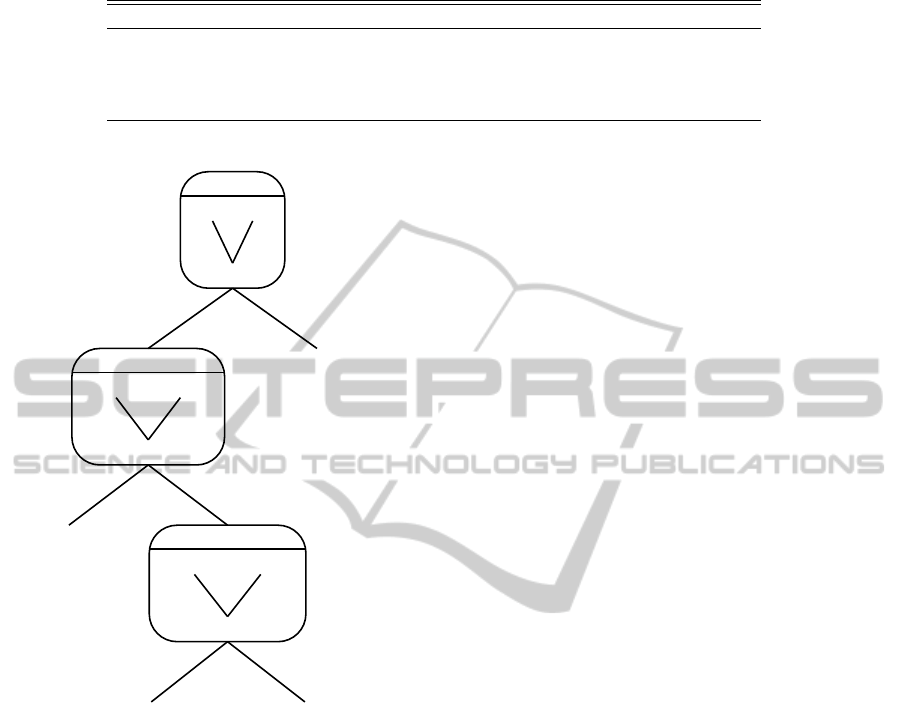
Table 1: Results for frequent subgraphs.

Algorithm Accuracy [%] Precision for incorrect proofs [%]

J48 97.2 98.8

SVM (SMO) 97.2 98.6

IB1 94.9 98.3

Naive Bayes 95.9 98.6

= TRUE

= FALSE

= TRUE

= FALSE

pattern1

{#}

{Z} {-Z}

pattern12

{Z}

{-X,Y,Z} {-Y,X}

negative (15.0)

pattern30

{-X}

{-X,Y,Z} {-Y,-Z}

negative (4.0) positive (330.0/9.0)

negative (44.0/1.0)

Figure 3: Decision tree with subgraphs as nodes.

Now let the total number of tree nodes be v, num-

ber of input trees n, the number of patterns found by

Sleuth m, the maximum number of patterns within a

single tree p, time complexity of Sleuth O





, time

complexity of sleuth results parsing O





, time com-

plexity of classiﬁer (building and testing) O





. Fur-

thermore, we can assume that m  p, m  n and

m  r. Then the total time complexity of 10-fold

cross validation is O



+ nmp + v + X +Y +C



5 DISCUSSION

5.1 Emerging Patterns

We also checked whether emerging patterns would

help to improve performance. All the frequent pat-

terns were ranked with GrowthRate metric (Dong and

Li, 1999) separately for each of the classes of cor-

rect and incorrect solutions. Because we aimed, most

of all, to recognize wrong resolution proofs, we built

two sets of emerging frequent patterns where the pat-

terns emerging for incorrect resolution proofs have

been added to the set of attributes with probability

between 0.5 and 0.8, and the emerging patterns for

the second class with probability 0.5 and 0.2, respec-

tively. Probability 0.5 stands for equilibrium between

both classes.

It was sufﬁcient to use only 10–100 top patterns

according to GrowthRate. The best result has been

reached for 50 patterns (generalized subgraphs) when

probability of choosing an emerging pattern for incor-

rect solution has been increased to 0.8. Overall accu-

racy overcome 97.5% and precision on the class of in-

correct solutions reached 98.8% with recall 87.3%. It

is necessary to stress that the number of attributes was

lower, only 50 to compare with 83 for experiments in

Table 1. We again used 10-fold cross validation.

5.2 Classiﬁcation into Three Classes

To increase precision on the class of incorrect proofs,

we decided to change the classiﬁcation paradigm and

allow the classiﬁer to leave some portion of exam-

ples unclassiﬁed. The main goal was to classify only

those examples for which the classiﬁer returned high

certainty (or probability) of assigning a class.

We used validation set (1/3 of learning examples)

for ﬁnding a threshold for minimal probability of clas-

siﬁcation that we accept. If the probability was lower,

we assigned class UNKNOWN to such an example.

Using 50 emerging patterns and threshold 0.6, we

reached precision on the class of incorrect solutions

99.1% with recall 81.6% which corresponds to 73 ex-

amples out of 90. It means that 17 examples were

not classiﬁed to any of those two classes, CORRECT

and INCORRECT solution. Overall accuracy, preci-

sion and recall for the correct solutions were 96.7%,

96.2% and 99.4%, respectively.

GraphMiningforAutomaticClassificationofLogicalProofs

567

5.3 Inductive Logic Programming

We also checked whether inductive logic program-

ming (ILP) can help to improve the performance un-

der the same conditions. To ensure it, we did not use

any domain knowledge predicates that would bring

extra knowledge. For that reason, the domain knowl-

edge contained only predicates common for the do-

main of graphs, like node/3, edge/3, resolutionStep/3

and path/2. We used Aleph system (Srinivasan, 2001).

The results were comparable with the method de-

scribed above.

6 CONCLUSION AND FUTURE

WORK

Our principal goal was to build a robust tool for

an automatic evaluation of resolution proofs that

would help teacher to classify student solutions.

We showed that with the use of machine learning

algorithms—namely decision trees and Support Vec-

tor Machines—we can reach both accuracy and pre-

cision higher than 97%. We showed that precision

can be even increased when small portion of exam-

ples was left unclassiﬁed.

The solution proposed is independent of a partic-

ular resolution proof. We observed that only about

30% of incorrect solutions can be recognize with a

simple full-text search. For the rest we need a solu-

tion that employs more sophisticated analytical tool.

We show that machine learning algorithms that use

frequent subgraphs as boolean features are sufﬁcient

for that task.

As future work we plan to use the results of this

system for printing report about a particular student

solution. It was observed, during the work on this

project, that even knowledge that is uncertain can be

useful for a teacher, and that such knowledge can be

extracted from output of the learning algorithms.

ACKNOWLEDGEMENTS

This work has been supported by Faculty of

Informatics, Masaryk University and the grant

CZ.1.07/2.2.00/28.0209 Computer-aided-teaching for

computational and constructional exercises. We

would like to thank Juraj Jur

co for his help with data

preparation.

REFERENCES

Brauner, B. (2013). Data mining in graphs. http://is.

muni.cz/th/255742/fi_b/.

Cook, D. J. and Holder, L. B. (2006). Mining Graph Data.

John Wiley & Sons.

Dong, G. and Li, J. (1999). Efﬁcient mining of emerging

patterns: Discovering trends and differences. pages

43–52.

Dovier, A., Pontelli, E., and Rossi, G. (2001). Set uniﬁca-

tion. CoRR, cs.LO/0110023.

GraphML team (2007). The graphml ﬁle format. http:

//graphml.graphdrawing.org/ [Accessed: 2014-

01-09].

Hall, M., Frank, E., Holmes, G., Pfahringer, B., Reutemann,

P., and Witten, I. H. (2009). The weka data min-

ing software: An update. SIGKDD Explor. Newsl.,

11(1):10–18.

Huan, J., Wang, W., and Prins, J. (2003). Efﬁcient mining of

frequent subgraphs in the presence of isomorphism. In

Proceedings of the Third IEEE International Confer-

ence on Data Mining, ICDM ’03, pages 549–, Wash-

ington, DC, USA. IEEE Computer Society.

Kerber, R., L. B. S. E. (1995). A hybrid system for data

mining. In Goonatilake, S., K. S., editor, Intelligent

Hybrid Systems, chapter 7, pages 121–142. Willey &

Sons.

Ketkar, N. S., Holder, L. B., and Cook, D. J. (2005). Sub-

due: Compression-based frequent pattern discovery in

graph data. In Proceedings of the 1st International

Workshop on Open Source Data Mining: Frequent

Pattern Mining Implementations, OSDM ’05, pages

71–76, New York, NY, USA. ACM.

Srinivasan, A. (2001). The Aleph Manual.

http://web.comlab.ox.ac.uk/oucl/research/

areas/machlearn/Aleph/ [Accessed: 2014-01-09].

Yan, X. and Han, J. (2002). gspan: Graph-based substruc-

ture pattern mining. In Proceedings of the 2002 IEEE

International Conference on Data Mining, ICDM ’02,

pages 721–, Washington, DC, USA. IEEE Computer

Society.

Zaki, M. J. (2005). Efﬁciently mining frequent embedded

unordered trees. Fundam. Inf., 66(1-2):33–52.

Zhang, Z. and Zhang, C. (2004). Agent-Based Hybrid Intel-

ligent Systems. SpringerVerlag.

Zhang, Z., Z. C. (2004). Agent-Based Hybrid Intelligent

Systems, chapter Agent-Based Hybrid Intelligent Sys-

tem for Data mining. In (Zhang and Zhang, 2004).

CSEDU2014-6thInternationalConferenceonComputerSupportedEducation

568