
Decision Support Tool for Group Job-shop Scheduling Problems
Yuri Mauergauz
Sophus Group, Leninski avenue 62, Moscow, Russia
Keywords: Production Scheduling, Decision Support Tool, Job-Shop, Simulation.
Abstract: This paper presents a new tool for group job-shop scheduling problems. The tool encompasses a dynamic
Pareto-optimal method based on two criteria simultaneously: relative setup expenditure criterion and
average orders utility criterion. In this method the concept of production intensity as a dynamic production
process parameter is used. The software used allows scheduling for medium quantity of jobs. The result of
software application is the set of non-dominant versions proposed to a user for making a final choice. Based
on this model, a decision support tool (DST) called OptJobShop is used for scheduling optimization. The
decision support tool provides for scheduling simulation with various initial parameters, comparison of
different scheduling versions and choice of the final decision.
1 INTRODUCTION
Technological grouping of jobs assures low setup
time for transition from a job to a job within a
group. For instance, if it is necessary to perform a
group of certain jobs (orders) to make one and the
same product on a single machine, a set of orders
turns into one batch for manufacturing. Such type
of grouping is typical for cutting, punching, plastic
details casting, etc., if the “make-to-order”
manufacturing strategy is used. In the other case, a
set of jobs may become a batch for manufacturing,
when all jobs have to be executed simultaneously
on a single machine (oven, bath).
Group scheduling is also applicable for the
“make-to-stock” manufacturing strategy, which is
typical for process manufacturing, production of
hardware, fasteners, general-purpose tools, etc. For
such production, as a rule, minimal product
quantity that is jointly manufactured is equal to a
“technical” lot. The latter depends on the machine
volume, package size, truckload value and so on.
From the economical point of view, it makes sense
to merge technical lots into batches, which may be
manufactured without a setup.
In the last two decades, a lot of papers
dedicated to group scheduling have been
published. Since group scheduling is a matter of
great computational complexity, every group
research, as a rule, was dedicated to a special
scheduling case, and seeks a scheduling solution
for the best value of certain criterion, for example
makespan
max
C
.
It is necessary to note, however, that the way a
group scheduling problem is formulated as a
problem with a single criterion contains an
inherent contradiction. Indeed, the main reason of
group scheduling is an attempt for rational tradeoff
between a high customer service level and a low
production cost. High customer service level
may be achieved only by timely order completion.
However, prompt order completion contradicts
requirement of keeping production expenses low.
Necessity to improve both characteristics
simultaneously is known as the “dilemma of
operation planning” (Nyhuis and Wiendal, 2009),
and its solution is in principle impossible with a
single criterion concept. More promising, but also
more complicated, will be a direction of research
seeking for Pareto-optimal diagrams on problem
criteria.
Apparently, to get the best solution for
“dilemma of operation planning”, one must design
Pareto-optimal diagrams on the basis of criteria,
which correspond to correlation between job
execution expenses and efficiency. As it was
shown in the paper by Mauergauz (2012), the
criterion of relative setup expenses
U and the
criterion of average orders utility
V
may be
considered for group scheduling. These criteria are
fundamental for computing of job-shop schedule
397
Mauergauz Y..
Decision Support Tool for Group Job-shop Scheduling Problems.
DOI: 10.5220/0004988903970406
In Proceedings of the 4th International Conference on Simulation and Modeling Methodologies, Technologies and Applications (SIMULTECH-2014),
pages 397-406
ISBN: 978-989-758-038-3
Copyright
c
2014 SCITEPRESS (Science and Technology Publications, Lda.)

both for “make-to-order” and “make-to-stock”
manufacturing strategies. The scheduling
simulation described in this paper provides a user
with a set of Pareto solutions for a final decision.
The remainder of this paper is organized as
follows. Section 2 provides a review of decision
support systems for manufacturing. In Section 3
the problem is formulated, the function of direct
expenses and the function of current orders utility
are determined. Section 4 is dedicated for the
structure of planning and decision support system.
The example of group job-shop modeling and
scheduling is described in Section 5. Section 6
includes discussion of results and outlook of
investigations.
2 DECISION SUPPORT
SYSTEMS FOR
MANUFACTURING
As far as the author knows, the paper by Viviers
(1983) was one of the early works, in which a
decision support system for job-shop scheduling
was used. To get suitable decision, the sequence of
jobs completion was set by an interactive user
interface. After a job was scheduled, a
corresponding due date based on the scheduled
lead time, was calculated. If work-in-process
volume and lead time values were not high, the
decision was supposed to be suitable.
Decision support systems designed in following
years differed by direction, structure and
simulation methods. The system’s goal is directly
connected with hierarchical level of planning that
the system is intended for. The most developed are
decision support systems for tactical long time
planning, when sales & operation plans are
designed. For example, the paper by Lee and Lee
(1999) was directed to coordination of
production/marketing decisions.
Mansouri et al. (2012) studied some decision
support problems in multi-criteria supply chain for
the MTO strategy. Barfod et al. (2011) designed
decision support system based on combining multi-
criteria decision analysis with cost-benefit analysis
both for production and transport aspects of
supply.
A number of systems were designed for
tactical long time planning on aggregated level.
The hierarchical decision support system by
Ozdamar et al. (1998) was integrated with MRP
system through Master Production Schedule. This
system had the interactive user interface for data
input and visualization of elaborated decision
versions. In the system designed for small
companies by Silva Filho and Cezarino (2007) MS
Access was used as a database. This system had a
constrained linear stochastic production planning
model. Silva et al. (2006) described the interactive
decision support system for an aggregate
production planning. A multi-criteria model with
mixed linear programming was developed for three
criteria: maximum profit, minimum late orders,
and minimum work force level changes. In the
work by Garcia-Sabater et al. (2009) the decision
support system for aggregate production planning
is concerned with determining the optimum
production, work force, and inventory levels for
each period of the planning horizon.
The important process in sales & operation
scheduling is inclusion of a new order into the
plan. In the paper by Okongwu et al. (2012) the
systems are described for estimation of order
inclusion expediency with regard to order
influence on the whole supply chain. Kalantari et
al. (2011) elaborated the decision support system
for order inclusion within MTS and MTO
strategies. The decision support systems review on
order inclusion was made in the paper by Slotnik
(2011).
Some systems are destined for decision
support in Master Production Scheduling. Fonseca
et al. (2005) designed the decision support system
for Master Production Scheduling for mass
production with the Just-in-Time. In the paper by
Silva (2009) the decision support system named
'PHIL' was described, which was intended for
regular week tasks in the synthetic fibre production
industry. Sotiris et al. (2008) designed the system
for weekly order releasing in metal forming
industry
.
Considerable number of decision support
systems that have been designed recently is
dedicated to daily scheduling. In these systems one
can make order release decisions and select
optimal parameters of production process. One of
the early order release systems was described by
Wang et al. (1994). In this paper, a neural network
approach is developed for order acceptance
decision support in job-shops with machine and
manpower capacity constraints. The order
acceptance decision problem was formulated as a
sequential multi-criteria decision problem. Oguz et
al. (2010) examined the order acceptance system,
where the orders were defined by their release
dates, due dates, setup times for a single machine.
SIMULTECH2014-4thInternationalConferenceonSimulationandModelingMethodologies,Technologiesand
Applications
398

Mahdavi et al (2010) elaborated the support system
for scheduling based on discrete events simulation.
The method “event – condition – action” was used
for decision making. In the paper by Hasan et al.
(2012) the decision support system for job-shop
scheduling was described, which used genetic
algorithm for makespan minimization.
In the more complex systems decisions are
supported on various planning levels. Such
systems may be divided into two groups. The
systems related to the first group may be used in
various industry fields; the systems related to the
second group are niche. For example, the system
VTT_GESIM (Heilala et al., 2010) has the general
destination. This system is based on methods of
Discrete Event Simulation. Such methods may be
applied for all kinds of discrete production,
including assembly and project production, and for
supply chains as well. Simulation may be made at
all production stages from design of the production
lines and the manufacturing cells to daily planning.
The feature of the system, which makes it possible
to apply in various fields, consists in special
parametrical files for database tuning. The system
(Kargin and Mironenko, 2009) is the example of a
niche system, which has the knowledge base and is
destined for sheet cutting at primary operation
shops.
Sometimes it is expedient to apply simpler
systems, which may be named as the decision
support tools. In the paper by Buehlmann et al.
(2000) the simple decision support system for
wood panel manufacturing is described. The
system consists of MS Excel forms, which make it
possible for a user in the shop to optimize the
schedule, as terms of supply and material prices
are changing. Novak and Ragsdale (2003)
elaborated a decision support methodology for
stochastic multi-criteria linear programming in MS
Excel. Petrovic et al. (2007) designed the decision
support tool using such linguistically quantified
statements as most, few etc. for estimation of batch
size influence, order importance and other
parameters as measure of plane quality. They
applied this tool in the pottery industry. In the
paper by Sakalli and Birgoren (2009) the decision
support tool for optimal receipt selection in brass
casting industry was described.
Such simple systems are useful, when it is
possible to use the available ERP-system for data
input and work lists making. In these cases the
decision support system has functions of
scheduling simulation, modification of initial
parameters for analysis and results visualization.
This paper suggests such a decision support tool
based on MS Excel for computing and final choice
of a multi-criteria group schedule in job-shops.
3 MAIN DEFINITIONS AND
PROBLEM FORMULATION
3.1 Utility Functions in Scheduling
The customer service level may be assessed by the
current order utility function V. From the
manufacturer’s point of view, the order value
increases proportionately to work amount
i
p
,
since staff engagement increases. Besides, the
more is the time reserve for completing an order,
the more attractive is the order, since there is an
opportunity to prepare for order execution.
Eventually the order time reserve is decreasing,
and the order value is diminishing. After all, if due
date has expired, the order value becomes
negative.
The manufacturer’s attitude to the order
changes in time and the appropriate function is
named production intensity (Mauergauz, 2012):
1
()/ 1
ii
i
i
wp
H
Gdt G
at
0
i
dt
and (1)
[( ) / 1]
ii
ii
wp
HtdG
G
at
0
i
dt
,
where:
i
p
= processing time of job i; G= plan bucket
duration;
i
w
= priority weight coefficient of job i;
= “psychological coefficient”;
i
d
= due date; t=
current time.
Figure 1: Production intensity diagrams.
DecisionSupportToolforGroupJob-shopSchedulingProblems
399

On abscissa axes in Figure 1 the time reserve is
measured. The reserve is equal to subtraction
between due date and current time. In the positive
part of the diagram (
i
dt
) the values of intensity
with growth of available time reserve decrease in
hyperbolic mode.
When the time reserve is negative (
i
dt
) and
there is delay of order completion, the production
intensity linearly increases. Since production
intensity is dimensionless it has no physical sense,
but it has psychological sense. Indeed, when this
order parameter is augmenting, the nervousness
about order execution is increasing. Two curves in
Figure 1 differ in the psychological coefficient
value. The higher is the
coefficient, the more
placid is the attitude to delays and the lower is the
intensity.
The production intensity concept may be used
for determination of the current order utility
function V (Figure 2).
Figure 2: Current order utility function.
Assume that the current utility for an order
i
is
ii
ii
wp
VH
G
.
(2)
The curve in Figure 2 for the positive value
0
i
dt
tends to the horizontal asymptote,
/
iii
VwpG
.
(3)
In the negative part
0
i
dt
the curve turns
into the inclined straight line with
i
tg
2
ii
wp
G
.
(4)
If the order due date reserve is positive, the
manufacturer usually intends to get some profit; if
reserve is negative and job execution delays the
manufacturer, as a rule, it incurs losses. There are
a great number of papers dedicated to the utility
changes as a function of available gain or loss.
Results of such researches may be reduced to one
of two versions depicted in Figure 3. On the
abscissa axis in Figure 3 the gain value (anticipated
profit
) is set, on the ordinate axis the gain
utility is set in the positive area of the abscissa
axis, and the loss utility - in the negative area. The
diagram 3a was named an S-mode curve as a result
of a well-known research by Kahneman and
Tversky awarded with the Nobel Prize on
economics in 2002. Their research proved
inclination of ordinary people to risk, when loss is
probable (the left part of the diagram). The left part
is concave, so a sign of corresponding second
derivative is positive, and there is risk proneness.
Figure 3: Possible diagrams of gain and loss utility; a) diagrams with risk averse and risk prone areas; b) diagrams only
with risk averse area.
0
0
V
V
L
o
s
s
b)
G
a
i
n
a)
L
o
s
s
G
a
i
n
SIMULTECH2014-4thInternationalConferenceonSimulationandModelingMethodologies,Technologiesand
Applications
400

In contrast to the diagram 3a, the diagram 3b
(Grayson-Bard utility function) shows risk
aversion both for gain or loss perspectives.
Difference of results in the diagrams 3a and 3b,
most probably, were caused by choice of people
circles for polling and by direction of money
application. In the research by Kahneman and
Tversky, modest people were interrogated,
money amounts were negligible, and their
purpose was consumption. On the contrary,
Grayson-Bard function was designed for
investments by large companies.
If we compare the curve in Figure 3 and the
curves in Figure 2, we can see that the order time
reserve is used as gain or loss. It seems to the
manufacturer that the long-term order
availability represents a considerable gain, but
the rate of this gain growth goes down in
proportion to the duration. In this positive field
the order utility curve behaves entirely like the
diagrams in Figure 3. The negative field in
Figure 2 is similar to the loss field in Figure 3,
but in contrast to the diagrams in Figure 3 there
is linear diminution of order utility function in
Figure 2. Accordingly, the function second
derivative is equal to zero, and risk is neutral.
Due to the additivity property of production
intensity and order utility function, it is possible
to compute the average utility of the whole order
set during a plan bucket. The value of this
parameter describes timeliness of order
completion and may be used as a criterion of
scheduling.
Let us assume that a certain job that
corresponds to the node of the scheduling
versions tree at the level
l
is completed at the
moment of time
l
C
. Let us also assume that the
job k with processing time
k
p
starts at the
moment
k
t
, which is more than or equal to
l
C
.
Then the average utility of the entire set of
jobs
J
from start until completion of the job k in
the node at the level
1l
equals
1,
0
11
()
kk kk
l
tp tp
lk l
lk
kk kk
C
VVdtVCVdt
tp tp
(5)
The function of negative expenses utility (loss
function) may be used as the second criterion in
the dilemma of operation planning. If the sequence
number of planning job is
n
, then
00
1
[()]
nn
s
li kl l
ll
UcsctC
c
,
(6)
where:
c= shift cost;
s
c
= hour setup cost;
i
c
= hour idle
cost;
kl
t
= moment of job k start after job l
completion;
l
s
= setup time for the next job with
the sequence number l in the specific schedule
version.
3.2 Planning Problem to Be
Considered
Let us consider the group job-shop problem. This
problem may be considered as scheduling for
several groups of parallel machines of various
purposes. In this case every job consists of a set of
operations, and every operation has to be executed
on a machine with a corresponding availability. Let
us assume that a set of jobs for manufacturing may
be divided into groups of several types, and
operation setup norms
ij
s
depend on the
corresponding machine group
j
and job kind i .
According to a planning system, which is used
at the plant, this problem has different versions. In
the simplest case one may suppose that at the
moment of planning the set of part batches to be
manufactured within a plan bucket (1-5 working
days) is known. In this case size of batches in
process of treatment does not change, therefore
release batches, transport batches and output
batches are equal.
The situation is much more complex, when the
kit planning system is applied. Within this system
a shop has to manufacture the specified number of
kits
k
n
consisting of different parts during a plan
bucket (for example, a working day). Besides,
different sets may include parts of one type. It is
also necessary to take into account that stocks for
parts of different parts may arrive to the shop at
various moments of time r
i
. If available criteria of
optimization are relative setup cost U and average
order utility
V
, in accordance with the well-
known three-part scheduling classification, the
considered problem is
|,,,|,
jikij
J
prec r n s U V
,
(7)
where:
DecisionSupportToolforGroupJob-shopSchedulingProblems
401

J
j
= machine quantity in a group j;
k
n
= needed
kit quantity on a day; r
i
= moment of stock arrival
;
i
j
s
= setup time; U = setup cost criterion;
V
=
average order utility criterion; prec = the
subsequent operation may be executed after all
previous operations.
There are two target functions in the formula
(7), and they may both be improved only within
certain limits. The Pareto compromise curve serves
as such limit, because in its points improvement
(reduction) of the criterion
U
is always related to
deterioration (reduction) of the criterion
V . To
solve the problem (7), we should apply a
MultiObject “Greedy” (MO-Greedy) algorithm
(Canon and Jeannot, 2011), which at every step
seeks a set of non-dominated solutions.
Examples of using this algorithm for group
multi-criteria scheduling are described in the paper
by Mauergauz (2013). With this approach for
every level of search tree constructional nodes of
non-dominated solutions should be found, and
then new
branches should grow from these nodes. Using the
formulas (1, 2, 5) and the rules for integral
calculations, we can compute the criterion
V
value in every node of the tree. The criterion
U
value may be computed by the formula (6) in every
node.
4 STRUCTURE OF PLANNING
AND DECISION SUPPORT
SYSTEM
The system to be considered consists of initial data
input, data preparation for planning, the
optimization model, the decision support tool and
visualization of computed results. The system
architecture and corresponding streams of
information are shown in Figure 4. The initial data
are being recorded on an MS Excel sheet by hand
or are transferred from ERP system. The VBA
program named OptJobShop provides the data
actuality, when planning begins and start of macros
with computer program for scheduling. The
planning results depend essentially on a number of
parameters. The simulation subsystem is the main
module of decision support, which makes it
possible to determine parameters influence.
The simulation parameters are input by a
graphical user interface. Parameters of branching
set constraints on nodes of the decision tree and are
being fixed during the system tuning. It is possible
to modify three main parameters of computing: the
psychological coefficient, size of the transport
batch and the planning horizon. The computation
results for various simulation parameters are being
recorded in an MS Excel sheet. After analysis of
criteria set for all scheduling versions the Gantt
diagram for selected version is being drawn.
Parameters of the selected version may be
transferred into the ERP system for generation of
working tasks.
Figure 4: The system architecture and information streams.
Data input to MS
Excel by hand or
transfer from ERP
system
OptJobShop
Data actualization when
planning begins
Scheduling start
Input of simulation
parameters
Analysis of results
Choice of the best decision
Optimization
program (MS
Excel macros
)
Gantt diagram
depiction
Computing of
working lists
SIMULTECH2014-4thInternationalConferenceonSimulationandModelingMethodologies,Technologiesand
Applications
402
5 EXAMPLE OF SYSTEM
USAGE
Let us consider an example of system usage.
Assume it is necessary to manufacture three types
of part kits in a shop. Assume also that the shop
must produce three kits of kind 1, one kit of kind 2
and two kits of kind 3 within a working day. Every
kit consists of parts of six types in any number. In
process of manufacturing parts of each type have
to be subjected to various technological operations
in a given sequence. Every operation may be
executed on the corresponding machine which
relates to a set of machines with similar
technological functions.
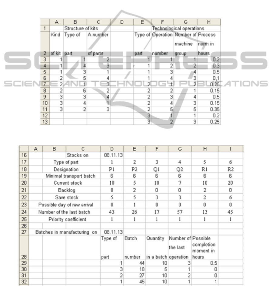
Figure 5 shows the record of composition of
sets and fragment of the operation table on the MS
Excel sheet. Figure 6 shows the records of
currents parts stocks and the records of parts
batches, which are in manufacturing at the moment
of planning.
Figure 5: Structure of kits and the table of operations.
Figure 6: Parts stocks and batches in manufacturing at the moment of planning.
DecisionSupportToolforGroupJob-shopSchedulingProblems
403
Apart from this data, information is recorded
onto an MS Excel sheet about number of machines
in each machine group, hour setup cost and hour
idle cost of these machines, information on every
machine setup on a moment of planning as well.
Setup norms for each technological operation and
working calendar for the several nearest days are
also recorded into the sheet. Let us assume that
during manufacturing every batch of parts is equal
to the minimal transport batch, which is given in
the stock table in Figure 6. After start of the
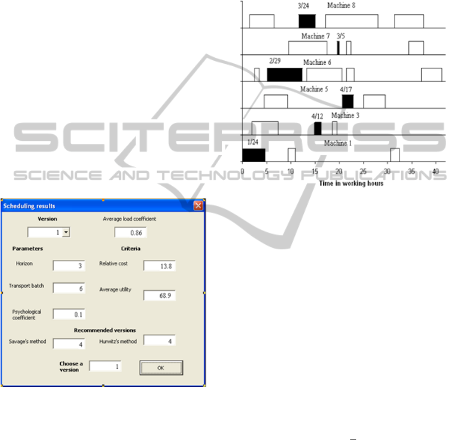
program the non-dominated decision versions are
being computed, and results have to be analyzed
with the graphical user interface shown in Figure
7. For each version the average load coefficient
and values of criteria are computed. The version
numbers, which are recommended for decisions by
Savage’s method and Hurwitz’s method, are
automatically determined and displayed on the
screen. Change of the simulation parameters
results in changes of scheduling criteria values.
The user can choose the version with criteria
values that are optimal in current situation.
Figure 7: Dialog support decision interface.
In Figure 8 the Gantt chart for a selected
version is shown. In this diagram the operations for
batches with parts of type 3 are marked in black.
At the beginning of scheduling in manufacturing
there is the batch No. 18 (Figure 6) with parts of
this type in amount of 5 pieces, and the last
completed operation for this batch is operation 1.
If one takes into account the available part stock,
backlog and save stock, to manufacture the
necessary kits within the horizon of 3 days, one
must complete this batch No. 18 and additionally
manufacture four transport batches of these parts.
As it is follows from Figure 8, for this purpose the
first operation has to be executed on the machine 1
with the release batch of 24 pieces. Then the
operation 2 is scheduled on the machine 6 for the
whole batch of 29 pieces.
Figure 8: Gantt chart for selected scheduling decision.
The operation 3 begins without waiting for
completion of all parts within the operation 2, so
24 parts are transported from the machine 6 to the
machine 8. Then the remainder has to be
transported to the similar machine 7. Some of
parts, which has been through the operation 3 in
amount of 12 pieces, must be transported to the
machine 3 for execution of the operation 4, and all
others in the amount of 17 pieces are joined on the
similar machine 5. Thus, automatically the
planning with parallel-consecutive treatment and
parts grouping into batches is realized.
6 CONCLUSION
We designed the decision support tool for dynamic
solution of the “operation planning dilemma” for a
job-shop. The relative setup cost
U
criterion and
the average orders utility
V
criterion are used to
define the correlation of “cost/efficiency” on the
planning horizon. The average orders utility value
is determined, depending on the production
intensity
i
H
of every order, which changes in
time. To design a schedule, a set of Pareto-optimal
solutions shall be calculated on the planning
horizon, and the final decision will be made by the
user.
SIMULTECH2014-4thInternationalConferenceonSimulationandModelingMethodologies,Technologiesand
Applications
404

The above results show that the group
scheduling approach, based on applying the
criterion of relative direct cost and the criterion of
average orders utility, allows computing the
satisfactory schedule versions. However, one
cannot assert that any version is the best within a
given set of versions and, all the more, within a
whole possible set of versions. Moreover, when the
planning horizon in the “make-to-stock” strategy is
changed, the computed schedule versions change
substantially as well. Quality of scheduling
depends essentially on initial parameters: size of
the transport batch, the planning horizon and the
psychological coefficient.
Computations show that the order utility is
great for a small transport batch. When the batch
size increases, the order utility diminishes. For the
numeral example in Section 5, in the interval from
6 to 12 pieces there is sharp decrease of the order
utility, then utility increases again. Thus, in this
case the optimal size of the transport batch is equal
to 6 or 12.
When the planning horizon changes, the
computed versions of schedule also change
substantially. If the horizon increases, the system
automatically offers the versions with larger
groups of transport batches. Computations show
that at the horizon that is named critical, the
number of output batches for parts of any type
begin to increase sharply. This horizon value may
be considered as maximum possible for
scheduling.
Scheduling is a regular process that repeats
with certain, but not always constant cycle. For
this purpose it is convenient to use new MS Excel
sheets, where information from previous sheets
may be contained. By changing or inserting of
new data, the user can correct the previous plan or
design a new one. The proposed decision support
tool gives possibility for transition from previous
date to subsequent one without serious changes in
the scheduling methodology.
In real practice various additional constraints
may be necessary for scheduling. For example,
often it is needed to take into account the current
device wear and tear, limited storage possibilities,
general shipping terms, etc. In our opinion, it is not
reasonable to take into account all such constraints
in a single program. For each case it is necessary
to create a special program with joint efforts of the
user and the main developer. In the nearest future it
is planned to elaborate some solutions, which
correspond to listed problems.
REFERENCES
Barfod MB, Salling K.B. and Leleur S. (2011).
Composite decision support by combining cost-
benefit and multi-criteria decision analysis. Decision
Support Systems, 51(1), 167-175.
Buehlmann, U., Ragsdale, C.T. and Gfeller, B. (2000). A
spreadsheet-based decision support system for wood
panel manufacturing. Decision Support Systems,
28(3), 207-227.
Canon, L.-C. and Jeannot, E. (2011). MO-Greedy: an
extended beam-search approach for solving a multi-
criteria scheduling problem on heterogeneous
machines. IEEE International Symposium on
Parallel and Distributed Processing Workshops and
PhD Forum, 57-69.
Garcia-Sabater, J.P. , Maheut, J. and Garcia-Sabater,
J.J.(2009). A decision support system for aggregate
production planning based on MILP: A case study
from the automotive industry. In Proceedings of the
International Conference on Computers & Industrial
Engineering, 366-371, Troyes.
Fonseca, D. J., Li, L. and Chen, D.-C. (2005). A
decision support system for production planning in
just-in-time manufacturing. Asian Journal of
Information Technology, 4(6), 623-627.
Hasan, S. M., Sarker, R. and Essam, D. (2012). A
decision support system for solving job-shop
scheduling problems using genetic algorithms.
Flexible Services and Manufacturing Journal, 23(2),
137-155.
Heilala J., Montonen J., Järvinen P., Kivikunnas S.
(2010). Decision support using simulation for
customer-driven nanufacturing system design and
operations planning. In Decision Support Systems,
Advances in, 235-260, Croatia, INTECH.
Kalantari, M., Rabbani, M. and Ebadian,M. (2011). A
decision support system for order
acceptance/rejection in hybrid MRS/MTO
production systems. Applied Mathematical
Modelling, 35(3), 1363-1377.
Kargin, A.A. and Mironenko, D. C. (2009). Concept
and algorithm model of imitation and simulation for
sheet cutting at primary operation shops of MZTM
plant. Donetsk National University Herald, Series
A, Natural sciences, 1, 452-457 (in Russian).
Lee, W.J. and Lee, K.C. (1999). A meta decision support
system approach to coordinating
production/marketing decisions. Decision Support
Systems, 25(3), 239-250.
Mauergauz, Y. (2012). Objectives and constraints in
advanced planning problems with regard to scale of
production output and plan hierarchical level.
International Journal of Industrial and Systems
Engineering, 12(4), 369-393.
Mauergauz, Y. (2013). Cost-efficiency method for
production scheduling. In Proceedings of the World
Congress on Engineering 2013, 587-593, London.
Mahdavi, I., Shirazi, B. and Solimanpur, M. (2010).
Development of a simulation-based decision support
DecisionSupportToolforGroupJob-shopSchedulingProblems
405

system for controlling stochastic flexible job shop
manufacturing systems. Simulation Modelling
Practice and Theory, 18, 768–786.
Mansouri S.A, Gallear D. and Askariazad M. H. (2012).
Decision support for build-to-order supply chain
management through multiobjective optimization.
International Journal of Production Economics
135(1), 24–36.
Novak, D.C. and Ragsdale,C.T. (2003) A decision
support methodology for stochastic multi-criteria
linear programming using spread sheets. Decision
Supports Systems. 36(1), 99-116.
Nyhuis, P. and Wiendal, H.P. (2009). Fundamentals of
Production Logistics. Springer, Berlin.
Oguz,C., Salman,F.S. and Yalcin, Z.B. (2010) Order
acceptance and scheduling decisions in make –to-
order systems. International Journal of Production
Economics, 125(1), 200-211.
Okongwu, U., Lauras, M., Dupont, L. and Humez, V.
(2012). A decision support system for optimising the
order fulfillment process. Production Planning &
Control, 23(8), 581-598.
Ozdamar, L., Bozyel, M. A. and Birbil, S. I. (1998). A
hierarchical decision support system for production
planning (with case study). European Journal of
Operational Research, 104(3), 403-422.
Petrovic, D., Duenas, A. and Petrovic, S. (2007)
Decision support tool for multi-objective jobshop
scheduling problems with linguistically quantified
decision functions. Decision Support Systems, 43(4),
1527-1538.
Sakalli, U.S. and Birgoren, B. (2009). A spreadsheet-
based decision support tool for blending problems in
brass casting industry. Computers & Industrial
Engineering, 56(2), 724-735.
Silva,C.G., Figueira, J., Lisboa, J. and Barman, S.
(2006). An interactive decision support system for an
aggregate production planning model based on
multiple criteria mixed integer linear programming.
Omega, International Journal of Management
Science, 34(2), 167-177.
Silva,C. (2009). Combining ad hoc decision-making
behaviour with formal planning and scheduling
rules: a case study in the synthetic fibre production
industry. Production Planning & Control, 20(7), 636
– 648.
Silva Filho, O.S and Cezarino, W. (2007 ). Managerial
decision support system for aggregate production
plan generation. In Proceedings of the 19
International Conference on Production Research,
Chile, Valparaiso, 1-6.
Slotnik, S.A.(2011). Order acceptance and scheduling: a
taxonomy and review. European Journal of
Operational Research, 212(1), pages 1-11.
Sotiris, G., Athanasios, S. and Ilias, T. (2008). A
decision support system for detailed production
scheduling in a Greek metal forming industry.
Management of International Business and
Economic Systems Transactions, 2(1), 41-59.
Viviers, F. (1983). A decision support system for job
shop scheduling. European Journal of Operational
Research, 14(1), 95-103.
Wang, J., Yang, J.Q. and Lee, H. (1994). Multicriteria
order acceptance decision support in over-demanded
job shops: a neural network approach. Mathematical
Computer Modeling, 19(5), l-19.
SIMULTECH2014-4thInternationalConferenceonSimulationandModelingMethodologies,Technologiesand
Applications
406
