High-Order Analytical Solution of Relative Motion Equation for Satellite
Formation Flying in Elliptical Orbit
Ting Wang
1
, Hanlun Lei
1
, Bo xu
1
, Tian Guan
2
and Jun Guo
2
1
School of Astronomy and Space Science, Nanjing University, 22, Hankou Road, Nanjing, Jiangsu Province, China
2
Mudra Intelligence Home Decorating Company,
No.8034, Plaza of International Home Decorating, Wuxi, 214000, China
Keywords:
Satellite Formation Flying, Elliptical Orbit, Periodic Configuration, Lindstedt-Poincare Method.
Abstract:
The paper studied relative motion equation for satellite formation flying with large separations. The configura-
tion is traditionally designed by the periodic solutions of the C-W equation in circle reference orbit or Lawden
equation in elliptic reference orbit. Hence, the linear solutions are more suitable for the configuration with
small scale formation than large scale formation. However, in some specific situations, it is necessary to use
satellites with large separations. Then the paper studied relative motion based on the nonlinear equations in an
elliptic reference orbit. The solution is expanded as series form with respect to the eccentricity of the reference
orbit, in-plane amplitude and out-of-plane amplitude. Taking the Lawden periodic solution as starting point,
the high-order analytical solution is constructed by Lindstedt-Poincare method. Particularly, as the eccentricity
is zero, the analytical solution degenerated to express the relative motion in circle reference orbit. Finally, the
practical convergence of the analytical solution is discussed in order to examine its validity and applicability.
1 INTRODUCTION
Multiple satellites form a certain configuration to
complete a common scientific exploration or task, the
mode of operation is called satellite formation flying.
Due to its potential technical advantages and widely
applications, the study of satellite formation flying is
more and more active in astronautics field. In fact, the
research on configuration is the essential and impor-
tant fundamental theory among formation flying tech-
nics, such as the dynamics, the capture, maintenance
and reconfiguration issues of satellite formation fly-
ing.
A successful satellite formation flying relies on
the technic of configuration. For example, to sus-
tain the formation, the economic fuel consumption is
related to the accuracy of the configuration. Gener-
ally, researchers used the linear Hill equation or C-W
equation, which is linearized the relative motion equa-
tion in a circular orbit. The analytical solution can
be directly derived. It is easy to be used to design
the configuration of satellites formation. However,
the analytical solutions of C-W equation are not ca-
pable to solve the problem as satellite’s formation has
a large separations. Therefore, the paper will gener-
ate high-order analytic solution in an elliptic reference
orbit based on the non-linear relative motion equa-
tion. The aim is to provide the precise mathematic
theory for the configuration,capture, reconfiguration,
and maintenance of satellite formation flying with a
large baseline in an elliptical orbit.
Relative motion problems can be considered as a
degenerate case of restricted three-body system, that
is, it corresponds to the specific situation when the
mass parameter of the three body system µ is 0. Thus,
the methods and results under the restricted three-
body system can be naturally applied to solve the
solution of the relative motion equations. In fact,
restricted three-body problem has abundant dynami-
cal properties, such as three collinear libration points
which are collinear with the main celestial have in-
stability dynamics quality. However, in most cases,
the other two triangular libration points which con-
stitutes an equilateral triangle with main celestial are
stable. Numerous researchers studied analytical solu-
tions of relative equation for satellite formation flying
both in an elliptical reference orbit and in a circle ref-
erence orbit. Richardson applied Lindstedt-Poincar’e
(L-P) method to derive the third-order analytic solu-
tion of Halo orbit near collinear libration points under
the circular restricted three-body system (Richard-
son.(1980)). Taking the analytical solution as the
256
Wang T., Lei H., Xu B., Guan T. and Guo J..
High-Order Analytical Solution of Relative Motion Equation for Satellite Formation Flying in Elliptical Orbit.
DOI: 10.5220/0004996902560263
In Proceedings of the 11th International Conference on Informatics in Control, Automation and Robotics (ICINCO-2014), pages 256-263
ISBN: 978-989-758-040-6
Copyright
c
 2014 SCITEPRESS (Science and Technology Publications, Lda.)

initial solution, more accurate numerical solution of
Halo orbit can be acquired by the differential correc-
tion method. Jorba and Masdemont expand Lissajous
orbit and Halo orbit near collinear libration points as
series form of in-plane amplitude and out-of-plane
amplitude. And they calculate coefficients corre-
sponding to every order solution (Jorba.(1999)).Since
the collinear libration points have unstable dynamic
properties, Masdemont expanded invariant manifolds
near libration points into series form of four am-
plitude parameters. Two of amplitudes corresponds
to hyperbolic manifolds, the other two amplitudes
are corresponding to the center manifold (Masde-
mont.(2005)). Taking into account the stable dynam-
ics properties of triangular libration points, the motion
in the vicinity of the triangular libration points can
be expanded to series form with respect to the long
period amplitude, short period amplitude and vertical
cycle amplitude, under the circle restricted three-body
system. Lei and Xu derive arbitrary high-order ana-
lytical solution which can provide a precise mathe-
matical tool for designing the missions near triangu-
lar libration points (Lei.(2013)). For the relative mo-
tion equation in the circle reference orbit, Richard-
son and Mitchell use L-P method to acquire a third-
order analytical solution (Richardson.(2003)). There-
after, G’omez and Marcote expand it to series solution
form of in-plane amplitude and out-of-plane ampli-
tude. It also used L-P method to bring arbitrary high-
order analytic solution (Gomez.(2006)). Ren et al de-
rived the third-order analytic solutions in the elliptical
reference orbit, and they explained how to generate
arbitrary high-order analytical solution (Ren.(2012)).
In this paper, the arbitrary high-order analytical so-
lution is generated by L-P method for relative mo-
tion of satellite formation flying with large baselines.
And the follower satellite’s relative motion can be ex-
pressed by series form related to orbital eccentricity
e, in-plane amplitude α and out-of-plane amplitude β.
From the elliptic restricted three-body problem,
the paper deduced the elliptical relative motion equa-
tion in the orbital coordinate. In the satellite for-
mation flying problem, the location of the chief cor-
responds to a libration point under degradation re-
stricted three-body system. Hence, the substantive
issue of configuration problem is to study dynamics
near libration points in the restricted three-body prob-
lem. With our existed work under the restricted three-
body system, in the orbital coordinate, the follower
satellite’s motion related to the chief satellite can be
expanded as series form of the orbital eccentricity
e, the in-plane amplitude α and out-of-plane ampli-
tude β. The arbitrary-order analytical solution can be
generated by the L-P method. Finally, we calculate
the convergence domain of high-order analytical so-
lution. In one hand, it verifies the validity of the anal-
ysis solution. On the other hand, it gives the scope of
the analytical solution according to the specific accu-
racy requirements.
The rest of paper is organized as follows. The dy-
namic model of the relative motion is introduced in
section 2. Based on the model and used L-P method,
the detailed procedures solving analytical solution is
described in the section 3. Section 4 analyzed the re-
sults of the solutions. Finally, some brief conclusions
were given in the last section.
2 THE ELLIPTICAL RELATIVE
MOTION EQUATION
Let us derive the elliptical relative motion equation
corresponding to an elliptical orbit from the perspec-
tive of the elliptic restricted three-body system. The
leader satellite P
1
is orbiting the Earth as an eccen-
tricity e elliptical motion. The follower satellite P
0
is
flying in the gravitational field produced by the Earth
and the leader satellite. Its motion is independent of
both the Earth and the leader satellite’s motion, such a
system is called an elliptic restricted three-body sys-
tem. The mass of the Earth, the chief satellite and the
follower satellite are respectively noted m
0
,m
1
,m
2
. In
the study, the dimensionless units are usually adopted.
The unit of mass is taken as the mass of the Earth and
the chief satellite, noted by [M] = m
0
+ m
1
; and Units
of length are the instantaneous distance between the
leader satellite and the earth, which is described as:
[L] = a(1 − e
2
/(1 + ecos f )), in which a is the orbit
semi-major axis, f is the chief satellite’s true anomaly;
to make the gravitational constant equal to 1, G = 1,
the time dimension is taken as:[T ] =
p
[L]
3
/(G[M]).
In the dimensionless system, the mass of the chief
satellite is expressed as µ = m
1
/(m
0
+ m
1
). Then the
mass of the Earth is expressed as 1 − µ.
For convenience, the coordinate origin located at
the centroid O of the Earth and the chief star. The unit
vector x is directed from the Earth to the chief satel-
lite. Z is positive in the direction of the instantaneous
angular momentum vector. Axis-Y is determined by
the right-handed coordinate system. The coordinate
system is called the barycenter synodic system O-
XYZ (see Fig. 1). In the barycenter synodic system,
the earth located at (µ,0,0) and the follower satellite
located at (1 − µ,0,0). The state vector is described
as (x, y, z, x
0
,y
0
,z
0
), where ∗
0
is
0
∗
0
partial derivatives
of true anomaly f, noted ∗
0
=
d∗
d f
. The dimensionless
relative motion equation of the follower satellite is as
High-OrderAnalyticalSolutionofRelativeMotionEquationforSatelliteFormationFlyinginEllipticalOrbit
257

Figure 1: Schematic diagram of barycenter synodic system
O-XY and orbital coordinate system o-xy.
follow:(Szebehely.(1967))





















¨
X −2
˙
Y =
1
1 + ecos f
∂Ω
∂X
¨
Y + 2
˙
X =
1
1 + ecos f
∂Ω
∂Y
¨
Z + Z =
1
1 + ecos f
∂Ω
∂Z
(1)
In Eq. 1, Ω is the potential function,
Ω =
1
2
(X
2
+Y
2
+ Z
2
) +
1 − µ
R
1
+
µ
R
2
. (2)
R
1
and R
2
are distances from P
2
to P
0
and from P
2
to
P
1
respectively,









R
1
=
q
(X +µ)
2
+Y
2
+ Z
2
R
2
=
q
(X −1 + µ)
2
+Y
2
+ Z
2
(3)
Eq.1 has five libration points, three of them are
collinear libration points located in the axis-X, de-
noted by L
i
, i = 1, 2, 3. The other two libration
points constitute equilateral triangle with the Earth
and the chief satellite. They are called triangle libra-
tion points, denoted by L
4
and L
5
.
In particular, for satellite formation flying prob-
lem, the mass of the chief satellite and the follower
satellite is approximately the same. However, their
masses are far less than the mass of the Earth. There-
fore, µ → 0. At the same time, in elliptic restricted
three-body problem, the collinear libration points L
1
and L
2
degenerate to a point, coinciding with the po-
sition of the chief satellite. In this case, the follower
satellite ’s relative motion converts to study the mo-
tion near collinear libration points corresponding to
µ = 0, in the elliptical restricted three-body problem.
It usually uses orbital coordinate system o-xyz (see
Fig. 1). The direction of axis is consistent with the
barycenter synodic system. The state vector is de-
noted by (x, y, z, x
0
,y
0
,z
0
). In the barycenter synodic
system, the chief satellite is located at (1,0,0), then
the coordinate transformation from orbital coordinate
system to the barycenter synodic system is expressed
as:
x = X −1,y = Y,z = Z. (4)
In orbital coordinate system, the follower satellite’s
relative motion is written as:





















¨x − 2 ˙y =
1
1 + ecos f
∂Ω
∂x
¨y + 2 ˙x =
1
1 + ecos f
∂Ω
∂y
¨z + z =
1
1 + ecos f
∂Ω
∂z
(5)
where Ω is ,
Ω =
1
2
(x
2
+ y
2
+ z
2
) +
1 − µ
R
1
+
µ
R
2
. (6)
r
1
is the distance between the follower satellite and
the Earth,
r
2
1
= (x + 1)
2
+ y
2
+ z
2
. (7)
Using the following formula, the relative motion
equation can be expressed as a polynomial form of
x, y and z.
1
p
(x − A)
2
+ (y − B)
2
+ (z −C)
2
=
1
D
∑
n≥0
(
ρ
D
)
n
P
n
(
Ax + By +Cz
Dρ
).
(8)
In Eq. 8, D
2
= A
2
+ B
2
+C
2
, ρ
2
= x
2
+ y
2
+ z
2
, P
n
is
Legendre polynomial, then
1
r
1
can be written as:
1
r
1
=
1
p
(x + 1)
2
+ y
2
+ z
2
=
∑
n≥0
ρ
n
P
n
(
−x
ρ
). (9)
Setting T
n
= ρ
n
P
n
(−
x
ρ
), R
n−1
=
1
y
∂T
n+1
∂y
, the following
relations can be described as:
∂T
n+1
∂x
= −(n + 1)T
n
,R
n−1
=
1
z
∂T
n+1
∂z
. (10)
T
n
and R
n
has the following recurrence relation,









T
n
=
1 − 2n
n
xT
n−1
−
n − 1
n
ρ
2
T
n−2
R
n
= −
2n + 3
n + 2
xR
n−1
−
2n + 2
n + 2
T
n
−
n + 1
n + 2
ρ
2
R
n−2
(11)
The initial values are T
0
= 1, T
1
= −x, R
0
= −1, R
1
=
3x. Substituting
1
1+ecos f
=
∑
i≥1
((−e)
i
cos f
i
) and Eq.
9 into Eq. 5, the relative motion equation in orbital
ICINCO2014-11thInternationalConferenceonInformaticsinControl,AutomationandRobotics
258

coordinate system can be rewritten as:



























¨x − 2 ˙y − 3x =
∑
i≥1
(3x · (−e)
i
cos f
i
) (12)
−
∑
i≥0
((−e)
i
cos f
i
)[
∑
n≥2
(n + 1)T
n
]
¨y + 2 ˙x =
∑
i≥0
((−e)
i
cos f
i
)[y
∑
n≥2
R
n+1
]
¨z + z =
∑
i≥0
((−e)
i
cos f
i
)[z
∑
n≥2
R
n+1
]
(13)
3 HIGH-ORDER ANALYTICAL
SOLUTION OF ELLIPTICAL
RELATIVE MOTION
EQUATION
3.1 High-order Expansion of Relative
Motion
Linearizing the relative motion Eq. 13 in orbital coor-
dinate, the following equations can be derived:











¨x − 2 ˙y − 3x = 3
∑
i≥1
(x · (−e)
i
cos f
i
)
¨y + 2 ˙x = 0
¨z + z = 0
(14)
The Eq.14 is the Lawden equation. Its periodic solu-
tion is the Lawdwn solution, which is expressed as:















x( f ) = α cos θ
1
+
1
2
αecos( f − θ
1
) +
1
2
αecos( f + θ
1
)
y( f ) = −2α sin θ
1
−
1
2
αesin( f + θ
1
)
z( f ) = β cos θ
2
(15)
In Eq.15, α and β are in-plane amplitude and out-of-
plane amplitude respectively. θ
1
and θ
2
are phase an-
gles. θ
10
and θ
20
are initial phase angles.
θ
1
= f + θ
10
,θ
2
= f + θ
20
. (16)
Considering the perturbation of the non-linear term,
the relative motion can be expanded as series solution
form, which is related to eccentricity, in-plane ampli-
tude, and out-of-plane amplitude.



















x( f ) =
∑
i, j,k,l,m,n
x
lmn
i jk
cos(l f + mθ
1
+ nθ
2
)e
i
α
j
β
k
y( f ) =
∑
i, j,k,l,m,n
y
lmn
i jk
cos(l f + mθ
1
+ nθ
2
)e
i
α
j
β
k
z( f ) =
∑
i, j,k,l,m,n
z
lmn
i jk
cos(l f + mθ
1
+ nθ
2
)e
i
α
j
β
k
(17)
In Eq.17, α and β are in-plane amplitude and out-
of-plane amplitude respectively. Phase angles are:
θ
1
= w f + θ
10
and θ
2
= w f + θ
20
. i, j,k ∈ N,l,m,n ∈
Z , and l, m, n have the same parity as i, j, k. In the
process of constructing the analytic solution, we only
need to consider coefficients that are satisfied with
following conditions: | l |≤ i, | m |≤ j and | n |≤ k .
As taking into account the symmetry of positive co-
sine function, supposing l ≥ 0; if l =0, then m ≥ 0 ; if
l=m=0, then n ≥ 0 . Similarly, the frequency can be
expanded as series solution in the form of the eccen-
tricity and the amplitudes.
w =
∑
i, j,k
w
i jk
e
i
α
j
β
k
(18)
Only when i, j, k are all even, the frequency coeffi-
cient w
i jk
is non-zero. Based on the Lawden solu-
tion Eq.15 , the arbitrary high-order solution of rela-
tive motion can be constructed by Lindstedt-Poincare
method.
The series solution Eq.17 is the analytical solu-
tion of the elliptical relative motion equation. If α 6=
0andβ = 0, Eq.17 describes the plane periodic config-
uration. If α = 0andβ 6= 0, it corresponds to the ver-
tical periodic configuration. Then if α 6= 0andβ 6= 0,
it depicts the general periodic configuration. Espe-
cially, if e=0, Eq.17 may degenerate to describe the
relative motion in circular reference orbit. In the pro-
cess of constructing the analytical solution, we define
two orders, represented by (N
1
,N
2
). N
1
= i is the or-
der corresponding to eccentricity, and N
2
= j +k is the
order corresponding to the amplitude. The total order
of the solution is N = N
1
+ N
2
. The order of Law-
den periodic solution is noted by (n
1
,n
2
), in which
n
1
= 1,n
2
= 1 , its corresponding known coefficients
can be expressed in detail as:









x
010
010
= 1.0,x
i−10
110
= 0.5,x
110
110
= 0.5
y
010
010
= −2.0,y
110
110
= −0.5
w
010
010
= 1.0,w
000
= 1.0
(19)
On the basis of Eq.19, the coefficients x
lmn
i jk
,y
lmn
i jk
,z
lmn
i jk
and w
i jk
corresponding to the high-order solution can
be solved by L-P method.
Coordinate system relating to the first and second
order partial derivatives of the true anomaly is:(take
component x as an example)





















˙x =
∂x
∂ f
+ w
∂x
∂θ
1
+ w
∂x
∂θ
2
(20)
¨x =
∂
2
x
∂ f
2
+ w
2
∂
2
x
∂θ
2
1
+ w
2
∂
2
x
∂θ
2
2
+ 2w
∂
2
x
∂ f wθ
1
+ 2w
∂
2
x
∂ f ∂θ
2
+2w
∂
2
x
∂θ
1
∂θ
2
(21)
High-OrderAnalyticalSolutionofRelativeMotionEquationforSatelliteFormationFlyinginEllipticalOrbit
259

To construct the analytical solution, it needs to distin-
guish known items from unknown items in the Eq.13.
For instance, the component x, its known items of
(n
1
,n
2
) order solution involves three parts. The first
part is corresponding to the right part of the relative
motion equation. The second part is from ˙y items
of the left part corresponding to the relative motion
equation. The last part stems from ¨x items corre-
sponding to the left part of the relative motion equa-
tion. Merge all known items into the right part of
the relative motion equation, denoted by X
lmn
i jk
. Sim-
ilarly, the known items of y and z corresponding
to the relative motion equation are denoted by Y
lmn
i jk
and Z
lmn
i jk
. Unknown coefficients of (n
1
,n
2
) order so-
lution includes (n
1
,n
2
) order coordinate coefficients
x
lmn
i jk
,y
lmn
i jk
,z
lmn
i jk
, and (n
1
,n
2
− 1) order frequency coef-
ficients w
i jk
.
In the relative motion equation corresponding to x
component, unknown items corresponding to (n
1
,n
2
)
order solution origin from ¨x , ˙y and x. And they are
respectively expressed as follows:









¨x → −(l + mw
0
+ nw
0
)
2
x
lmn
i jk
− 2w
0
w
i j−lk
δ
l0
δ
m1
δ
n0
˙y → (l + mw
0
+ nw
0
)y
lmn
i jk
− 2w
i j−lk
δ
l0
δ
m1
δ
n0
x → x
lmn
i jk
,i = n
1
, j + k = n
2
(22)
In the relative motion equation corresponding to y
component, unknown items are from ¨y , ˙x, they are
respectively written as:





¨y → −(l + mw
0
+ nw
0
)
2
y
lmn
i jk
+ 4w
0
w
i j−lk
δ
l0
δ
m1
δ
n0
˙x → −(l + mw
0
+ nw
0
)x
lmn
i jk
− w
i j−lk
δ
l0
δ
m1
δ
n0
(23)
In the relative motion equation corresponding to z
component, unknown items are from ¨z , z, they are
respectively written as:





¨z → −(l + mw
0
+ nw
0
)
2
z
lmn
i jk
− 2w
0
w
i j−lk
δ
l0
δ
m1
δ
n0
˙z → z
lmn
i jk
,i = n
1
, j + k = n
2
(24)
The L-P method requires that the same order item
must be equal on both sides of the equation. There-
fore, the equation of the unknown coefficients can be
established as:











A
1
x
lmn
i jk
+ B
1
y
lmn
i jk
+C
1
w
i j−lk
δ
l0
δ
m1
δ
n0
= X
lmn
i jk
A
2
x
lmn
i jk
+ B
2
y
lmn
i jk
+C
2
w
i j−lk
δ
l0
δ
m1
δ
n0
= Y
lmn
i jk
(−ψ
2
+ 1)z
lmn
i jk
− 2w
0
w
i j−lk
δ
l0
δ
m1
δ
n0
= Z
lmn
i jk
(25)
In Eq. 25, δ
i j
is the Dirac symbol. If i=j, then δ
i j
=
1, otherwise, δ
i j
= 0. Denoted ψ = l + mw
0
+ nw
0
,
A
i
,B
i
andC
i
,i = 1, 2 are:





A
1
= −(ψ
2
+ 3),B
1
= −2ψ,C
1
= (4 − 2w
0
)
A
2
= −2ψ,B
2
= −ψ
2
,C
2
= (4w
0
− 2)
(26)
3.2 High-order Solution for Solving the
Corresponding Coefficient
In Eq. 25, four unknown coefficients need to
be solved. For (n
1
,n
2
) order solution, three sub-
equations all contain unknown frequency coefficient
w
i jk
, j + k = n
2
− 1. Thus, the equation correspond-
ing to z component should be solved firstly. Then, cal-
culate coefficients corresponding to z coordinate and
frequency coefficients. At last, substituting the fre-
quency coefficients into the equation corresponding
to x-y component in order to solve coordinate coeffi-
cients corresponding to x and y.
3.2.1 Solving the Equation Corresponding to z
Component
Case 1: If | ψ |= 1
Case 1.1: If l=0, m=0, n=1, in this case, −ψ
2
+
1 = 0. Setting z
lmn
i jk
= 0, it can be solved that
w
i jk−1
= −
Z
lmn
i jk
2
.
Case 1.2: others, setting z
lmn
i jk
.
Case 2: if | ψ |6= 1, in this case, the unique un-
known coefficient is z
lmn
i jk
, then z
lmn
i jk
=
z
lmn
i jk
−ψ
2
+1
.
3.2.2 Solving the Equation Corresponding to x-y
Component
Since w
lmn
i jk
, j +k = n
2
−1 is known, the unknown co-
efficients are only x
lmn
i jk
and y
lmn
i jk
, and they are solved
in the following cases:
Case 1: if | l |= 1
Case 1.1: If ψ = 1, setting x
lmn
i jk
= 0, y
lmn
i jk
= −
X
lmn
i jk
2
.
Case 1.2: If ψ = 0, setting x
lmn
i jk
= 0, y
lmn
i jk
= 0, then
x
lmn
i jk
= −
X
lmn
i jk
3
.
Case 1.3: others, the unknown coefficients x
lmn
i jk
and y
lmn
i jk
are satisfied with the following equation:





−(ψ
2
+ 3)x
lmn
i jk
− 2ψy
lmn
i jk
= X
lmn
i jk
−2ψx
lmn
i jk
− ψ
2
y
lmn
i jk
= Y
lmn
i jk
(27)
ICINCO2014-11thInternationalConferenceonInformaticsinControl,AutomationandRobotics
260

Case 2: if l=0
Case 2.1: If m=1, n=0,Setting x
lmn
i jk
= 0 in order to
solve y
lmn
i jk
. (Or setting y + i jk
lmn
= 0 in order to
calculate x
lmn
i jk
). Taking the former case, then
y
lmn
i jk
= −
[X
lmn
i jk
− (4 − 2w
0
)w
i j−lk
]
2
. (28)
Case 2.2: if m + n = 0, in this case, y
lmn
i jk
are co-
efficients of sin(0). Setting y
lmn
i jk
= 0, then x
lmn
i jk
=
−
X
lmn
i jk
3
.
Case 2.3: if | m + n |= 1 and m 6= 1, setting x
lmn
i jk
,
then y
lmn
i jk
= −
X
lmn
i jk
2(m+n)
.
Case 2.4: others, the unknown coefficients satisfy
the following equation:





−((m + n)
2
+ 3)x
lmn
i jk
− 2(m + n)y
lmn
i jk
= X
lmn
i jk
−2(m + n)x
lmn
i jk
− (m + n)
2
y
lmn
i jk
= Y
lmn
i jk
(29)
In summary, the corresponding coordinates and fre-
quency coefficients of arbitrary high-order analytical
solution can be solved.
4 RESULTS
Using the Fortran program, the arbitrary high-order
solution is constructed, and coefficients of the (3, 3)
order solution is listed in Table 1. It showed that all
of frequencies coefficients are zero except ω
000
= 1.
That is, frequency of the relative motion are neither
related to the reference orbital eccentricity nor the
amplitude of the formation. The frequency is always
1.0, indicating that the relative motion is a periodic
configuration of 2π. As mentioned, Eq.17 can de-
scribe the general periodic configuration in the vicin-
ity of the chief satellite. Taking (7,10) order solu-
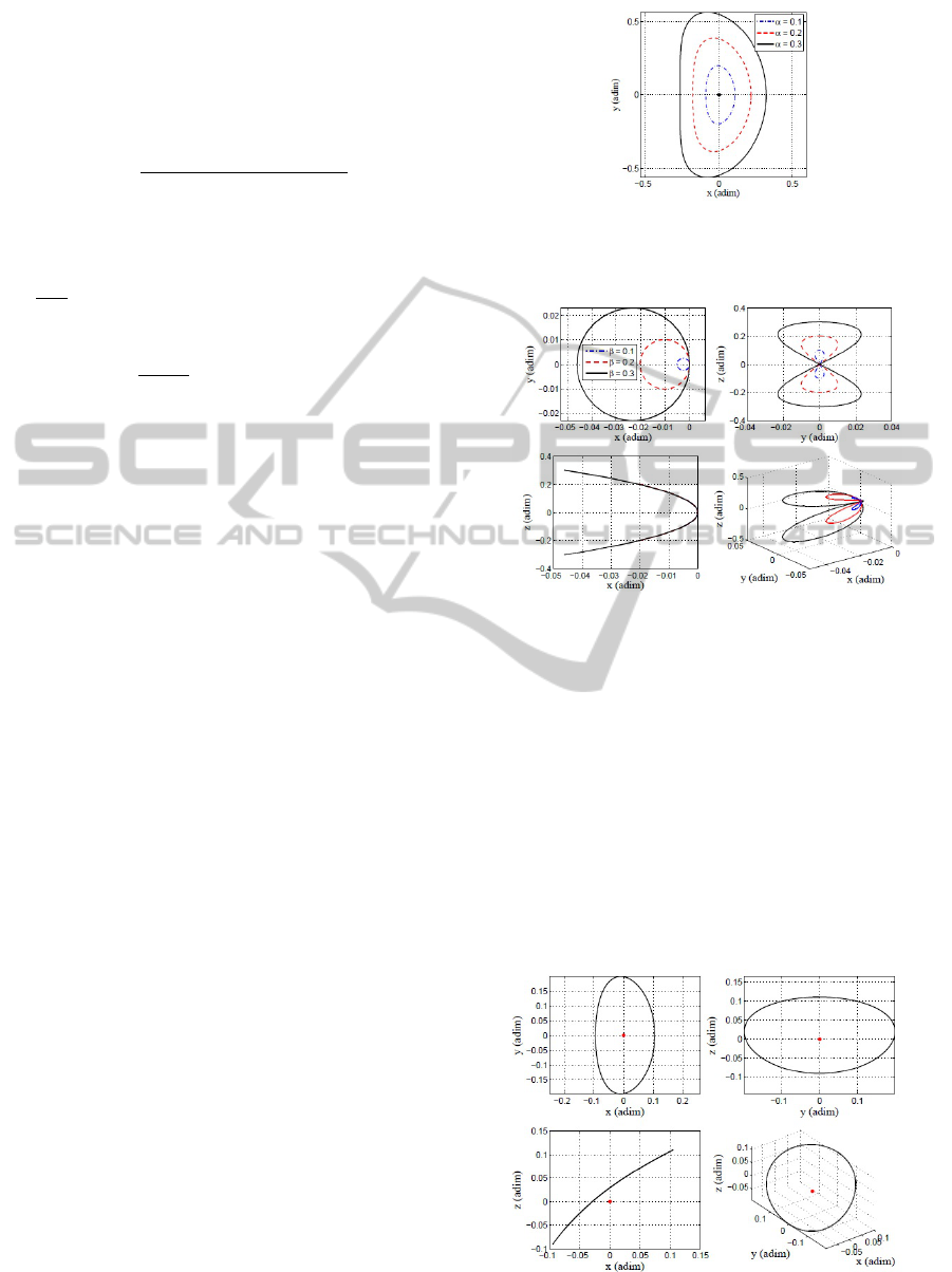
tion as an example, Fig.2 shows the plane periodic
orbits with (e = 0.1), β = 0, α = 0.1,0.2,0.3adim.
Fig.3 shows the vertical periodic orbits with (e = 0.1),
α = 0, β = 0.1,0.2,0.3adim. Fig.4 shows the periodic
orbit with e = α = β = 0.1. As e = 0, the solution 17
can describe the periodic orbit corresponding to circu-
lar reference orbit. Fig.5 showed plane periodic orbits
with e=0, α = 0.2,β = 0,computed by series expan-
sions up to order (0, 15). Fig. 6 showed vertical peri-
odic orbits with e = 0, α = 0, β = 0.2,computed by se-
ries expansions up to order (0,15). Fig. 7 showed the
periodic orbits with e=0, α = 0.2,β = 0.2,computed
by series expansions up to order (0,15). In all figures,
Figure 2: Plane periodic orbits with e = 0.1, α =
0.1,0.2, 0.3,β = 0,computed by series expansions up to or-
der (7,10).
Figure 3: vertical periodic orbits with (e = 0.1), α = 0,
β = 0.1, 0.2,0.3adim, computed by series expansions up to
order (7,10).
the given ’adim’ are dimensionless unit of length that
is instantaneous distance between the chief satellite
and the Earth.
In addition, combining numerical integration
methods, the scope and the convergence range of an-
alytic solution is illustrated. In the analytical solution
Eq.17 has three parameters , namely the reference or-
bital eccentricity e, the in-plane amplitude α and the
out-of-plane amplitude β. If e is fixed ( i.e e = 0.1 )
, the paper studied the convergence range of in-plane
amplitude and out-of-plane amplitude. The results of
Figure 4: Periodic orbits with e = α = β = 0.1, computed
by series expansions up to order (7,10).
High-OrderAnalyticalSolutionofRelativeMotionEquationforSatelliteFormationFlyinginEllipticalOrbit
261

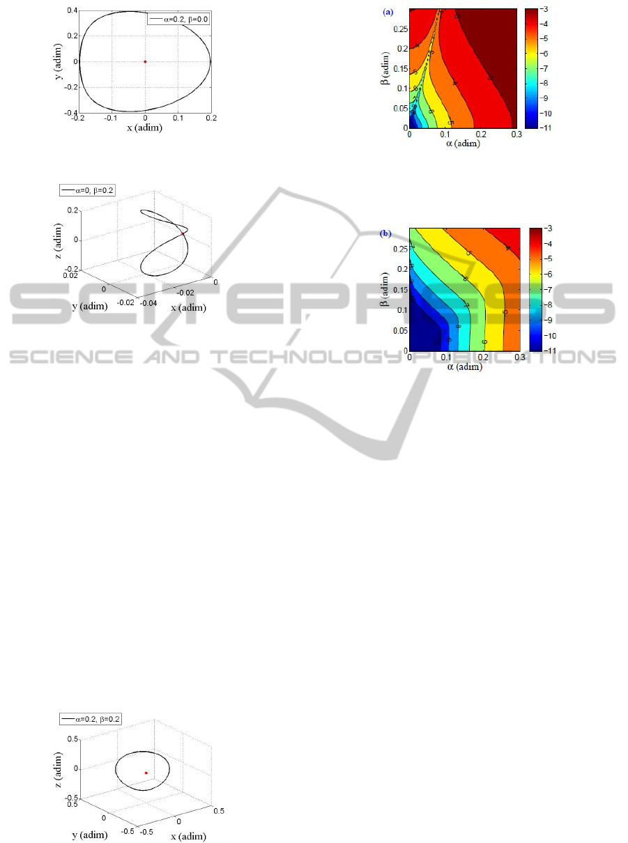
Figure 5: Plane periodic orbits with e=0, α = 0.2,β =
0,computed by series expansions up to order (0,15).
Figure 6: Vertical periodic orbits with e=0, α = 0,β =
0.2,computed by series expansions up to order (0,15).
( 5,5 ) order and ( 7,10 ) order analytical solutions
have been displayed. In the computing process, the
max in-plane amplitude and the max out-of-plane am-
plitude are both 0.3 adim. In the region [0, α
max
] ×
[0,β
max
], it is uniformly divided into 100 × 100 grids.
Each grid referred to a set (α,β), represented as (i, j),
and the corresponding set of amplitude is denoted by
(α
i
,β
j
),i = 1,2,...100; j = 1,2,...100. For each (i, j),
the state vectors can be obtained by analytical solution
Eq.17. Taking the state vectors as the initial value,
the relative motion Eq.5 integrate may de integrated
through the integrator RKF78 from f = 0 to f = 2π.
The position vector corresponding to f = 2π is rep-
resented as X
N
. Meanwhile, the analytical solution
17 can directly derive the position vector, denoted by
X
A
. Thus , as f = 2π, the position difference from the
numerical solution to analytic solution is denoted by
d
i j
=| X
A
− X
N
|. If the difference is smaller, it means
that the analytical solution is more accurate. Fig.8 and
Fig. 9 illustrate the convergence range of (5, 5) order
and (7,10) order respectively. In both figures, the pre-
Figure 7: The periodic orbits with e=0, α = 0.2,β =
0.2,computed by series expansions up to order (0,15).
Figure 8: The practical convergence of the high-order an-
alytical solutions of the equations of relative motion with
elliptic reference orbit, corresponds to the analytical solu-
tions truncated at order (5,5).
Figure 9: The practical convergence of the high-order ana-
lytical solutions of the equations of relative motion with el-
liptic reference orbit,corresponds to the analytical solutions
truncated at order (7,10).
cision coordinates are ln d
i j
. Obviously, if the order is
larger, the convergence range of analytical solution is
greater.
Due to computational efficiency and problem of
computer memory, the constructed order of analyti-
cal solution is limited. However, taking into account
the e, α and β and appropriate adjusting n
1
and n
2
in the order (n
1
,n
2
), the optimal configuration can be
acquired according to specific accuracy requirements.
For example, constructing analytical solution of cir-
cular orbit, n
1
does not contributed to the accuracy
since e = 0. Supposing n
1
= 0, the higher order ana-
lytical solution can be constructed by choosing higher
n
2
order.
5 CONCLUSIONS
The paper firstly derived the relative motion equation
in an elliptical reference orbit under restricted three-
body problem. Then the relative motion equation is
linearized in order to obtain the Lawden and Lawden
periodic solution. Taking into account the nonlinear
term of the relative motion, the motion in the vicin-
ity of the chief satellite is expanded as series form of
orbital eccentricity, the in-plane amplitude and out-
ICINCO2014-11thInternationalConferenceonInformaticsinControl,AutomationandRobotics
262

of-plane amplitude. Adopting Lawden solution as
the initial solution, the arbitrary high-order analyti-
cal solution is generated by using Lindstedt-Poincar’e
method. From results, it can be concluded that the
frequency of periodic configuration is always equal to
1.0, that is, the orbital period of the relative motion is
always 2π. It can be applied to the control and recon-
figuration of the satellite formation flying with large
baseline.
REFERENCES
Richardson D L. Analytic construction of periodic orbits
about the collinear points. Celest Mech, 22: 241C253,
1980.
Jorba A‘ , Masdemont J. Dynamics in the center manifold of
the collinear points of the restricted three body prob-
lem. Physica D, 132:189C213, 1999.
Masdemont J J. High-order expansions of invariant mani-
folds of libration point orbits with application to mis-
sion design. Dyn Syst, 20:59C113, 2005.
Lei H L, Xu B. High-order analytical solutions around trian-
gular libration points in circular restricted three-body
problem. Mon Not R Astron Soc,434: 1376C1386,
2013.
Richardson D L, Mitchell J W. A third-Order Analytical So-
lution for Relative Motion with a Circular Reference
Orbit. J Astron Sci, 51:1C12, 2003.
Gomez G, Marcote M. High-order analytical solutions
of Hills equations. Celest Mech Dyn Astron, 94:
197C211, 2006.
Ren Y, Masdemont J J, MarcoteMet al. Computation of an-
alytical solutions of the relative motion about a Ke-
plerian elliptic orbit. Acta Astronaut, 81: 186C199,
2012.
Szebehely V. Theory of orbits. New York: Academic Press,
1967.
APPENDIX
Table 1: The coefficients of coordinate series of the analyt-
ical solution constructed up to order (3,3).
i j k l m n x
lmn
i jk
y
lmn
i jk
z
lmn
i jk
0 0 1 0 0 1 0.0000 0.0000 1.0000
0 1 0 0 1 0 1.0000 -2.0000 0.0000
0 0 2 0 0 2 -0.2500 0.2500 0.0000
0 0 2 0 0 0 -0.2500 0.0000 0.0000
0 1 1 0 1 1 0.0000 0.0000 -0.5000
0 1 1 0 1 -1 0.0000 0.0000 1.5000
0 2 0 0 2 0 0.5000 0.2500 0.0000
0 2 0 0 0 0 -0.5000 0.0000 0.0000
0 1 2 0 1 2 0.1250 -0.1250 0.0000
0 1 2 0 1 -2 0.0000 0.3750 0.0000
0 2 1 0 2 1 0.0000 0.0000 0.3750
0 3 0 0 3 0 -0.3750 -0.2917 0.0000
0 3 0 0 1 0 0.0000 1.1250 0.0000
1 1 0 1 1 0 0.5000 -0.5000 0.0000
1 1 0 1 -1 0 0.5000 0.0000 0.0000
1 2 0 1 2 0 0.1250 0.0000 0.0000
1 2 0 1 0 0 0.0000 0.7500 0.0000
1 1 2 1 1 0 0.2500 -0.2500 0.0000
1 1 2 1 1 -2 0.3125 0.0000 0.0000
1 1 2 1 -1 2 0.2500 -0.2500 0.0000
1 1 2 1 -1 0 0.2500 0.0000 0.0000
1 1 2 1 -1 -2 0.0625 0.0625 0.0000
1 2 1 1 2 1 0.0000 0.0000 0.0625
1 2 1 1 2 -1 0.0000 0.0000 0.3125
1 2 1 1 0 1 0.0000 0.0000 0.5000
1 2 1 1 0 -1 0.0000 0.0000 -1.5000
1 2 1 1 -2 1 0.0000 0.0000 -0.3750
1 2 1 1 -2 -1 0.0000 0.0000 0.1250
1 3 0 1 3 0 -0.1667 -0.1042 0.0000
1 3 0 1 1 0 -0.7500 0.0000 0.0000
1 3 0 1 -1 0 0.6875 0.0000 0.0000
1 3 0 1 -3 0 -0.1458 0.0417 0.0000
2 2 0 2 -2 0 0.1250 0.0000 0.0000
2 2 0 0 2 0 0.0625 -0.0625 0.0000
2 2 0 0 0 0 -0.0625 0.0000 0.0000
2 3 0 2 3 0 -0.0208 -0.0104 0.0000
2 3 0 2 1 0 -0.1250 0.0000 0.0000
2 3 0 2 -1 0 0.0000 -0.1875 0.0000
2 3 0 0 3 0 -0.313 0.0104 0.0000
2 3 0 0 1 0 0.0000 -0.1875 0.0000
3 3 0 3 -3 0 0.0208 0.0000 0.0000
3 3 0 1 1 0 -0.0938 0.0938 0.0000
3 3 0 1 -1 0 -0.1094 0.0000 0.0000
3 3 0 1 -3 0 0.0052 0.0052 0.0000
High-OrderAnalyticalSolutionofRelativeMotionEquationforSatelliteFormationFlyinginEllipticalOrbit
263