Approximate Distance Queries for Path-planning in Massive Point

Clouds

David Eriksson and Evan Shellshear

Fraunhofer-Chalmers Centre, Gothenburg, 412 88, Sweden

Keywords:

Point Clouds, Distance Computation, Path-Planning, Simpliﬁcation.

Abstract:

In this paper, algorithms have been developed that are capable of efﬁciently pre-processing massive point

clouds for the rapid computation of the shortest distance between a point cloud and other objects (e.g. tri-

angulated, point-based, etc.). This is achieved by exploiting fast distance computations between specially

structured subsets of a simpliﬁed point cloud and the other object. This approach works for massive point

clouds even with a small amount of RAM and was able to speed up the computations, on average, by almost

two orders of magnitude. Given only 8 GB of RAM, this resulted in shortest distance computations of 30

frames per second for a point cloud originally having 1 billion points. The ﬁndings and implementations will

have a direct impact for the many companies that want to perform path-planning applications through massive

point clouds since the algorithms are able to produce real-time distance computations on a standard PC.

1 INTRODUCTION

High-resolution point clouds have become very im-

portant in the last decades as researchers have started

to exploit their advantages over triangle-based mod-

els in computer graphics applications (Tafuri et al.,

2012), (Sankaranarayanan et al., 2007). Improve-

ments in scanning technologies make it possible to

easily scan very large objects, thereby making point

clouds more popular than CAD models in certain ap-

plications. This is because point clouds offer the

user the ability to acquire valid representations of the

real state of the environment under consideration and

not just the nominal or planned appearance (Berlin,

2002). Scanned point cloud models are also able to

provide up-to-date information about local changes,

which is often much easier to acquire than updating

a given CAD model. Most importantly, however, for

industrial settings that lack a CAD (or similar) model,

one can scan an entire factory much easier than build-

ing a new CAD model from scratch.

One area where point clouds are useful is in path-

planning, where the core algorithms are based on col-

lision detection and/or the computation of the shortest

distance between a point cloud and an object moving

through the point cloud. The processing and efﬁcient

structuring of massive point clouds is critical in order

to speed-up path-planning algorithms, (Pauly et al.,

2002). The reason for this is that computing the nec-

essary collisions and/or distances is a common bottle-

neck for path-planning algorithms (Bialkowski et al.,

2013).

In certain scenarios, the point clouds used for

path-planning can contain billions of points, (Fr¨ohlich

and Mettenleiter, 2004), making it a challenge to pro-

cess them efﬁciently. Volvo Cars have scanned their

factories in Torslanda with the resulting point cloud

containing 10 billion points, (Volvo, 2013).

Path-planning through environments consisting of

triangle meshes has been studied intensively and there

exists a signiﬁcant amount research on the subject

(LaValle, 2006), (Latombe, 1990), (Carlson et al.,

2013), (Spensieri et al., 2013), (Spensieri et al., 2008)

and (Hermansson et al., 2012). Although the area of

path-planning with point clouds is newer, there are

methods designed speciﬁcally for it, such as (Landa,

2008) and (Landa et al., 2007). Path-planning through

hybrid environments has also been considered, where

the geometry is a point cloud and the object to be

path-planned is a triangle mesh; such combinations

havebeen studied in (Tafuri et al., 2012), (Sucan et al.,

2010) and (Pan et al., 2011). Hybrid path-planning is

uncommon because of the possibility to triangulate

the point cloud and use path-planning on the result-

ing triangle meshes, (Dupuis et al., 2008). However,

this triangulation process is only of interest for point

clouds smaller than those considered in this paper, for

which the usual algorithms used to triangulate point

Eriksson D. and Shellshear E..

Approximate Distance Queries for Path-planning in Massive Point Clouds.

DOI: 10.5220/0005002000200028

In Proceedings of the 11th International Conference on Informatics in Control, Automation and Robotics (ICINCO-2014), pages 20-28

ISBN: 978-989-758-040-6

 2014 SCITEPRESS (Science and Technology Publications, Lda.)

clouds would be far too cumbersome to be practical,

(Tafuri et al., 2012).

Path-planning can be approached from two dif-

ferent directions either via using collision queries or

distance queries. In this article we focus on path-

planning algorithms that require a fast distance com-

putation. Our results demonstrate the possibility of

speeding up distance queries in order to make path-

planning for massive point clouds feasible. By using

distance queries it is possible to provide more robust

results when path-planning in point clouds such as in

the aforementioned virtual Volvo Cars factory. In ad-

dition, in real life, designers have tolerances and error

margins built into their designs that need to be taken

into account when path-planning. Such concerns can

easily be managed by basing path-planning on com-

puting distances. On the other hand, by using distance

based path-planners we can also exploit these error

margins to speed up distance computations. If the de-

signer has an error of a couple of centimeters in their

models, then it is possible to speed up distance queries

because we know that millimeter accuracy is not nec-

essary. With this insight and new ways of using data

structures for distance queries, we are able to speed

up distance computations for massive point clouds by

almost two orders of magnitude. We also present two

theorems guaranteeing that our algorithm performs as

desired. To the best of the author’s knowledge, these

two theorems do not exist in the literature.

This paper is structured as follows: Section 2 will

describe how a simpliﬁed point cloud can be created

given a maximal allowed error in the computed short-

est distance. We also prove that the proposed sim-

pliﬁcation methods produce an error in the distance

queries that can be controlled by the level of simpli-

ﬁcation. Section 3 explains how the simpliﬁed point

cloud can be divided into subsets to expedite distance

computations. Section 4 explains how to compute the

shortest distance between the simpliﬁed point cloud

subsets and the path-planning object based on these

subsets. Section 5 evaluates the algorithms by consid-

ering a real-world point cloud and triangulated geom-

etry. In the ﬁnal section we conclude. The results in

this paper are based on the work in (Eriksson, 2014).

2 SIMPLIFICATION OF THE

POINT CLOUD

In order to be able to work more efﬁciently with a

massive point cloud, it would be beneﬁcial to create

a simpliﬁcation of the point cloud with fewer points.

The fewer points such a representation has, the faster

the distance computations will be. Hence, we look for

an appropriate trade-off between a slightly incorrect

but much faster distance computation.

2.1 Notation

To prepare for later results, some notation is neces-

sary. The point cloud will always be denoted by P

and its corresponding cardinality (number of points)

by |P|, which will be assumed to be ﬁnite. The point

cloud consists of a set of points in R

and this paper

will focus on n = 2 or n = 3 unless stated otherwise.

Denote by p

, i = 1, 2, . . . , n, the coordinates of a point

p ∈ R

and let p

, p

, . . . , p

denote m points where

∈ R

. When a subset of P is considered it will be

denoted by Q, i.e. Q ⊆ P. Multiple disjoint subsets

of P will be denoted by Q

and when no particular

subset is of interest the index will be dropped. The

object that will be moved through the point cloud will

be denoted by S, and it will be a compact subset of

We now give a central deﬁnition that plays an im-

portant role in the rest of the paper, that of the distance

between objects.

Deﬁnition 1. Let Q, R ⊂ R

and for q ∈ R

let kqk

stand for the Euclidean norm. Deﬁne:

d(q, r) = kq−rk,

d(q, R) = inf

r∈R

d(q, r),

d(Q, R) = inf

q∈Q

r∈R

d(q, r),

(Q, R) = max

(

sup

q∈Q

inf

r∈R

d(q, r), sup

r∈R

inf

q∈Q

d(q, r)

)

whereby the ﬁnal distance deﬁnition is the well-

known Hausdorff metric. The next deﬁnition deﬁnes

what is meant by a simpliﬁcation of a point cloud.

Deﬁnition 2. For ε ∈R

a point cloud P

is referred

to as an ε-simpliﬁcation of P if it satisﬁes:

1. |P

| ≤ |P|

2. d

(P, P

) ≤ ε .

The ﬁrst condition means that an ε-simpliﬁcation

can never have more points than the original point

cloud. The second condition means that for all points

in the original point cloud P, there should be a point

in the ε-simpliﬁcation near it and also that we do not

create new points in the ε-simpliﬁcation of P that are

far away from points in the original cloud P. Both

these conditions seem very natural. In Section 2.4 we

will show that the second requirement implies the de-

sirable condition that

|d(P, R) −d(P

, R)| ≤ ε, ∀R ⊆ R

. (1)

ApproximateDistanceQueriesforPath-planninginMassivePointClouds

We now present two simpliﬁcation methods that ful-

ﬁll Deﬁnition 2. Note also that one could attempt a

simpler down-sampling, however, for our applications

we need to guarantee that the down-sampling satisﬁes

Equation 1 and it is not so obvious how to produce an

efﬁcient down-sampling that fulﬁlls this requirement.

2.2 The Grid-based Partitioning

The ﬁrst ε-simpliﬁcation scheme presented here is

based on partitioning the point cloud by small axis-

aligned grid boxes with diagonal 2ε, with ε ∈ R

When simplifying the point cloud, two points that are

closer than 2ε may be represented by the midpoint of

the line connecting them in P

without violating Equa-

tion 2 in Deﬁnition 2. The grid-based partitioning uti-

lizes this fact by partitioning the original bounding

box of the point cloud into disjoint axis-aligned grid

boxes with side length

√

ε so that the diagonal of

each grid box is 2ε. All points that fall into the same

axis-aligned grid box may be represented by the box’s

midpoint in P

. In order to allow for this partitioning,

the original bounding box of P can easily be extended

to make all side lengths divisible by

√

ε. Extending

the bounding box will still guarantee that it contains

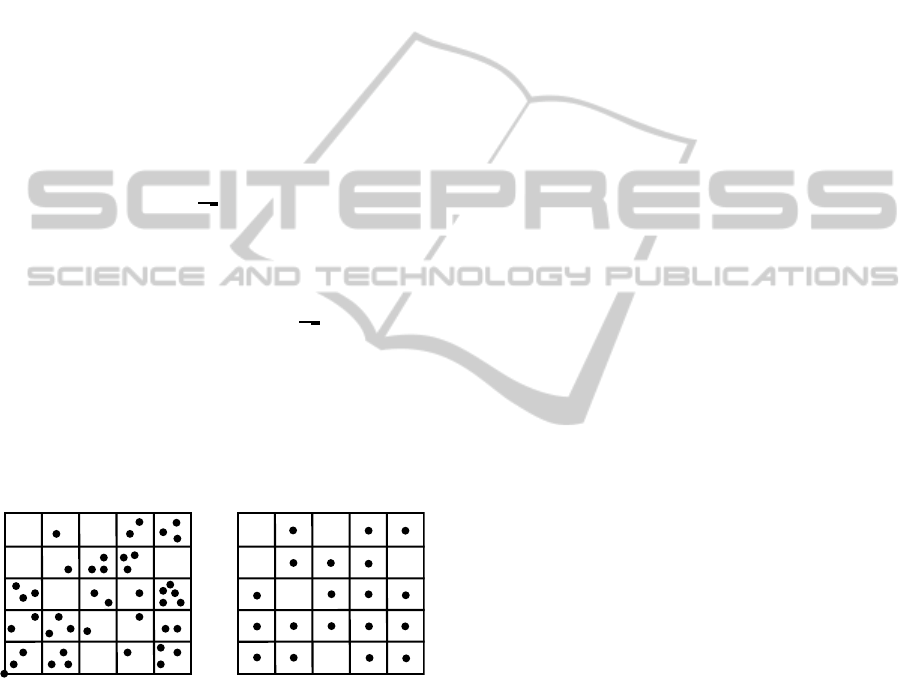
The simpliﬁcation scheme is illustrated in Figure

1 where the original point cloud in 2D can be seen

to the left and the resulting simpliﬁed point cloud

obtained from using the grid-based partitioning ε-

simpliﬁcation can be seen to the right.

Figure 1: (Left) Original 2D point cloud. (Right) ε-

simpliﬁcation of the point cloud after using the grid-based

partitioning.

Note that it is possible that |P

| = |P| if only one

point falls within each axis-aligned grid box, which

could happen if the point cloud is sparse or if ε is

very small. In addition, it is obvious that such a

simpliﬁcation method fulﬁlls our deﬁnition of an ε-

simpliﬁcation.

2.3 The k-means Method

The grid-based partitioning described in the previ-

ous section has the advantage of having linear time-

complexity in the size of the point cloud, but it may

give a non-optimal partitioning for at least two rea-

sons:

1. A box of diagonal 2ε can be contained in a sphere

with radius ε.

2. The position of the axis-aligned grid boxes is cho-

sen based only on the bounding box of P and no

other properties of the point cloud

The ﬁrst point addresses the fact that an axis-aligned

grid box of diagonal 2ε is not the object of maximal

volume that can be used to simplify a set of points.

In fact, Equation 2 of Deﬁnition 2 will also hold in

the case when all points falling within a sphere with

radius ε are represented by the center of the sphere.

The location of the spheres will depend on the distri-

bution of the point cloud since the original bounding

box cannot be partitioned into disjoint spheres.

This also addresses the second problem of the

grid-based partitioning, which concerns the fact that

the axis-aligned grid boxes placement only depends

on the bounding box of P and not on the structure of

the point cloud. Taking the distribution of points into

account is expected to make it possible to create an

ε-simpliﬁcation with a smaller |P

One way of placing the spheres adaptively is to

use k-means clustering. The k-means method is one

of the oldest clustering methods whose aim is to di-

vide a set of points into k clusters. The algorithm

is based on work by Lloyd, (Lloyd, 1982), and is

often referred to as Lloyd’s algorithm. The clusters

, . . . ,C

have the properties C

⊆ Q, C

∩C

0 for

i 6= j, and

i=1

= Q. Each cluster has a centroid µ

which is computed as the the mean value of all points

belonging to cluster C

. A point is assigned to the

cluster with the centroid closest to the point. The k-

means method for a set of points Q can be written as

the optimization problem:

minimize

,...,C

∑

j=1

∑

i∈C

−µ

, ∀q

∈ Q. (2)

The k-means method can be used to divide the

point cloud recursively. For each new subset it has

to be investigated whether the radius of the smallest

enclosing sphere has a radius that is no more than ε.

If the radius is larger than ε, the k-means method can

be used to create new clusters until each cluster can

be represented by the center of a sphere with radius

of at most ε. An optimal k-means method is expected

to produce a better clustering than the grid-based par-

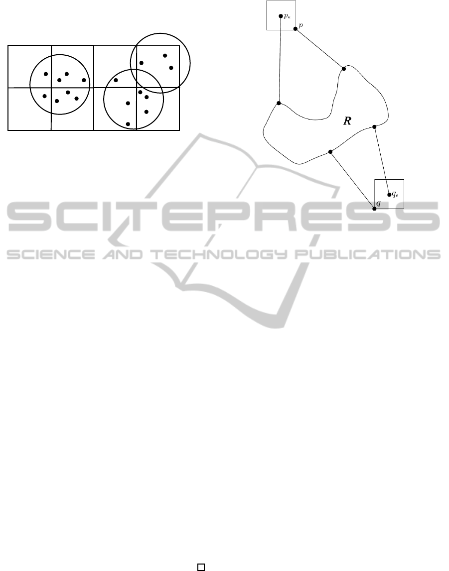
titioning as is illustrated in Figure 2.

As with the grid-based simpliﬁcation it is possible

that |P

| = |P| if ε is small in comparison to the distri-

bution of points. Otherwise it is obvious that such a

ICINCO2014-11thInternationalConferenceonInformaticsinControl,AutomationandRobotics

simpliﬁcation method also fulﬁlls our deﬁnition of an

ε-simpliﬁcation.

Figure 2: Grid based method compared to the k-means

method in 2D, illustrating that the k-means method may be

able to create a simpliﬁed point cloud with fewer points.

2.4 Maximum Error In the Computed

Shortest Distance

This section will show that Condition 2 of Deﬁnition

2 implies Equation 1. This is trivial if P consists of

only one point and follows directly from the trian-

gle inequality, see Figure 3. The following theorem

shows that the error in the shortest distance is always

bounded by ε for an ε-simpliﬁcation scheme satisfy-

ing Deﬁnition 2.

Theorem 1. Let P be a point cloud and let P

be an

ε-simpliﬁcation of P and let R ⊆ R

. Then it follows

that

|d(P, R) −d(P

, R)| ≤ ε (3)

Proof. Let p = argmin

y∈P

d(y, R) and let p

∈ P

such that d(p, p

) ≤ ε. It follows that

d(p

, R) ≤ d(p, p

) + d(p, R) ≤ ε+ d(p, R). (4)

Let q

= argmin

y∈P

d(y, R). Then,

d(q

, R) ≤ d(p

, R) ≤ ε+ d(p, R). (5)

In addition, there exists a point q ∈ P such that

d(q, q

) ≤ ε. Hence,

d(q, R) ≤ d(q, q

) + d(q

, R) ≤ ε + d(q

, R) (6)

and as before we have

d(p, R) ≤d(q, R) ≤ ε+ d(q

, R). (7)

Hence from Equations 5 and 7 it follows that,

|d(P, R) −d(P

, R)| ≤ ε. (8)

Figure 3: Illustration of the maximal error in Theorem 1 in

the case of simplifying with grid boxes with diagonal 2ε.

3 ORGANIZING THE POINT

CLOUD FOR FAST DISTANCE

QUERIES

This section explains how the original bounding box

of the point cloud will be successively divided and

organized into new disjoint sub-boxes in order to ob-

tain a partitioning of the original point cloud for fast

out-of-core distance queries. These subsets of points

make it possible to carry out distance queries for large

point clouds given only a small amount of main mem-

ory.

Given the original point cloud, it is straightfor-

ward to ﬁnd the bounding box of P. Suppose that we

want to divide the point cloud into subsets of at most

T points and that |P| > T. By splitting the original

bounding box along one of the coordinate directions

two new sub-boxes can be created. The sub-boxes

are divided into two new sub-boxes recursively until

all subsets contain no more than T points. Note that

there are several options for dividing the sub-boxes,

such as along the longest side or the coordinate direc-

tion with the largest variance. Each method of subdi-

vision affects the quality of the data structures that are

based on these sub-boxes and we chose to split in the

coordinate direction with the largest variance. Split-

ting in this direction seemed to produce good results

although more thorough tests are required to investi-

gate the relationship between splitting choice and per-

formance results.

We choose the value of T so that numerous sub-

ApproximateDistanceQueriesforPath-planninginMassivePointClouds

sets of points can ﬁt in main memory but also so that

each subset has a large number of points so we mini-

mize the number of reads from hard disk. At the same

time, by choosing T so that we have numerous sub-

sets, we can then exploit this by carrying out the dis-

tance queries to each of these subsets in parallel. We

explore the effects of different values of T in Section

5. The choice of T obviously depends signiﬁcantly on

the disk transfer rate (SSD vs HDD) and our choices

are optimized for our chosen hardware.

4 DISTANCE COMPUTATION

This section describes how the distance from a sub-

set to the object can be computed quickly in-core. It

introduces the Proximity Query Package (PQP) and

also derives a necessary condition in order to deter-

mine when a subset can contain the point closest to

the object in the point cloud considered.

4.1 Proximity Query Package

A fast way to ﬁnd the shortest distance between a

point cloud and a triangulated or point-based object

is needed in order to be able to compute distances

to the subsets that may contain the closest point. In

order to do so we chose to use PQP which was de-

signed for collision detection, distance computation,

and tolerance veriﬁcation between pairs of geomet-

ric models, (Larsen et al., 1999). It has been shown

to be the best choice of bounding volume hierarchy

for distance queries when fast queries are the goal,

(Larsen et al., 1999), (Lauterbach et al., 2010). PQP

uses swept sphere volumes to create a bounding vol-

ume hierarchy that can be used to efﬁciently compute

the shortest distance by traversing the tree of bound-

ing volumes.

The memory requirement to build a single PQP

model is signiﬁcant since building a PQP model with

1 billion points uses about 36GB of RAM. This mem-

ory limitation is not a problem for the proposed ap-

proach due to our memory-based management of the

PQP models, which will store numerous small PQP

models out of core. Hence each subset of points will

have one PQP model, so if T is chosen small enough

each individual PQP model can be built without using

much memory and can easily be stored out-of-core

and read into main memory quickly as disk transfer

time is often the bottleneck (see (Eriksson, 2014) for

more results).

4.2 STXXL

The Standard Template Library for Extra Large Data

Sets (STXXL) is an implementation of the C++ stan-

dard template library for external memory (out-of-

core) computations. The point cloud will be stored

in an STXXL vector (Dementiev et al., 2008) during

the simpliﬁcation phase. However, using STXXL im-

poses some limitations on users such as only being

able to hold so-called plain old data structures (ints,

ﬂoats, doubles, etc.) as elements in a STXXL vec-

tor, (Dementiev et al., 2008). It is also not allowed to

use references or pointers to elements in an STXXL

vector since elements are temporarily read into mem-

ory when requested, so that references will get invali-

dated when elements are evicted from memory. These

limitations makes the construction of a single out-of-

core PQP model with STXXL problematic. In addi-

tion, the implementation of an out-of-core PQP data

structure is not desirable because the changes would

require abandoning the advantageous C++ program-

ming paradigm to implement all data structures as

plain old data structures. Another reason is that RAM

accesses are about one order of magnitude faster than

memory accesses using STXXL when data has to be

read from the disk.

In order to avoid considering all subsets for each

distance query, Theorem 2 in the next section will pro-

vide a necessary condition for a subset to contain the

point closest to the object. The PQP models that are

closest will be kept in-core and PQP models that are

far away will remain on the hard disk, in cases where

all PQP models may not ﬁt in-core. This situation can

change when the object moves, in which case some

PQP models will have to be loaded while others will

have to be removed from main memory in case all of

the PQP models cannot ﬁt at once.

To achieve this, PQP was modiﬁed to allow writ-

ing of the interior data structure in a binary format to

the hard disk. Note that it is difﬁcult to apply such

a method to a single large PQP model and use it to

only read in parts of the hierarchy on an as needed

basis. This is because when querying a bounding vol-

ume hierarchy it is unknown which parts of the hi-

erarchy will be required and accesses can be largely

random. In the current case, with smaller individual

models and the coming Theorem 2, we are able to

avoid this problem. Because of this, it was decided

to write each PQP model to the hard drive by using a

binary format and then reload them when needed.

An advantage with this modiﬁcation is that the

distance computation can be carried out in parallel,

which would not have been the case if an STXXL vec-

tor of it had been used to hold the PQP models. An-

ICINCO2014-11thInternationalConferenceonInformaticsinControl,AutomationandRobotics

other advantage with not using STXXL is that when

a PQP model has to be read, PQP models that are far

away from S can be removed since they are not ex-

pected to be used again. In the case of using STXXL

it is not clear what will be removed in order to free up

the space for the reading.

4.3 A Fast Exclusion Theorem

In this section a very simple criterion is constructed

to make it possible to exclude a majority of the point

subsets without computing any distances when it is

clear that they are too far away from the object S

to contain the closest point. First we describe what

is meant by a motion of the object that we wish to

move through the point cloud. The object S will

be moved via rigid body motions M(t), i.e. transla-

tions and rotations. A conﬁguration of S is denoted

by S(t) := M(t)S, which is the position of S at time

t. Assume that the shortest distance is computed at

times t

where t

= 0 and S = S(t

). If p ∈ S is a

point that originally belongs to S, then we denote

this point at time t after rotations and translations by

p(t) := M(t)p. Note that p never moves with respect

to S. Some deﬁnitions are necessary before stating the

fast exclusion theorem:

Deﬁnition 3. Deﬁne by α

an upper bound on the

largest displacement of S between t

i−1

and t

, that is

= max

p∈S

kp(t

) −p(t

i−1

))k. (9)

Deﬁnition 4. Deﬁne d

min

(t) to be the shortest dis-

tance from the object S(t) to the point cloud P at time

The idea is that α

can be used to bound how much

closer a subset can be to the object compared to the

previous iteration. The result is stated in the following

Theorem:

Theorem 2. Let P be a point cloud and divide P

into m disjoint subsets. Let i ≥ 1, j ∈ {1, . . . , m} and

i−1

) be a lower bound on the distance from subset

j to S(t

i−1

). Then no point in subset j can be closer

to S(t

) than

max(0, d

i−1

) −α

) (10)

and also

d(P, S) ≤ d

min

i−1

) + α

. (11)

Proof. The ﬁrst statement follows from the fact that

the object has moved at most α

and that no point

in point subset j was closer than d

i−1

) before S

moved, which yields that no points in the subset can

be closer than max(0, d

i−1

) −α

). Since the object

has moved at most α

, the point that was previously

at a distance d

min

i−1

) away cannot be further away

than d

min

i−1

) + α

. This implies the second state-

ment.

The theorem makes it possible to neglect a large

amount of the subsets that are known to be too far

away to contain the point closest to the object. The

idea is to compute the initial values d

(0) before the

object starts moving. Similarly, an upper bound on

min

(0) can be computed by considering only a few

points per subset and save the shortest distance found.

The use of the theorem is illustrated in Algorithm 1.

Algorithm 1: Computation of the shortest distance using

Theorem 2.

for subset number j do

Compute an initial lower bound of d

(0)

end for

Find an upper bound for d

min

(0)

i ←1

while Object is moving do

Move S to the next position and compute α

min

) ← d

min

i−1

) + α

for each subset number j do

) ← d

i−1

) −α

if d

) ≤ d

min

) then

Compute d

) using the PQP model

Set d

min

) = min(d

), d

min

))

end if

end for

i ← i+ 1

end while

This inequality based on α

is designed for quick

evaluation, however it should be mentioned that it can

be very weak in the sense that it does not take the

direction of movement into account. If the object is

moved away from a subset so that the distance from

the points in subset j to the object increases, the lower

bound will be pessimistic since α

will be subtracted

from d

i−1

) .

5 SIMULATION RESULTS

The point cloud that will be considered is a part of

a factory and consists of about 1 billion points. In

this section of the factory a car chassis is required to

move from a start to an end conﬁguration. In addi-

tion, it is often required that the car be at least a given

distance from the surrounding point cloud along the

whole path. A picture of the point cloud can be seen

in Figure 4. The object will be moved from the hub

in the upper right corner to the hub in the lower left

ApproximateDistanceQueriesforPath-planninginMassivePointClouds

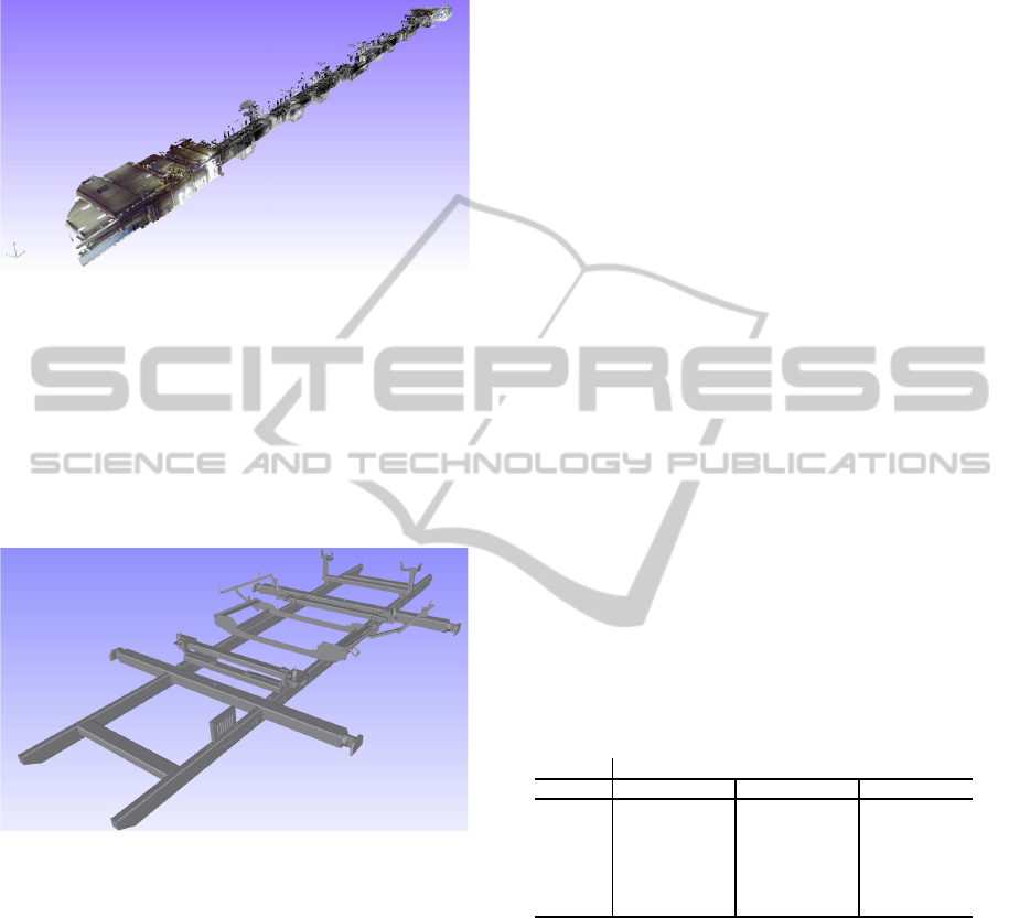
corner of Figure 4 along a known path. There are a

total of 700 discrete time steps. The spacing between

points in the point cloud is about 0.5 centimeters.

Figure 4: An overview of the original point cloud consisting

of about 1 billion points.

The object that is moved through the point cloud

is a holding mechanism for a car and its triangulation

consists of 78,403 triangles and can be seen in Figure

5. The position of the object along the path is given

at discrete points in time and the displacements of the

object vary in size. The variation in the displacements

will directly affect the computed values of α

Figure 5: A visualization of the object, a car holding mech-

anism, that will be moved through the point cloud.

To compute α

we computedthe originalbounding

box of the object S and transformed its eight corners at

each iteration and then computed the furthest a corner

point had moved and set that equal to α

. In the case

of no rotations of the object this upper bound is in fact

exact.

The computer used for the simulations was an In-

tel Core i7 processor, 32 GB RAM, and a 250 GB

SSD. The amount of RAM was constrained to 8 GB

in order to force the algorithms to run out-of-core for

the original point cloud with 1 billion points. In the

ﬁrst step we built PQP models for both the triangu-

lated object S and the point cloud considered. If all

points are stored as triplets of ﬂoats, the total memory

requirement for all the point cloud PQP models equals

36 GB, so that only at most 22% of the PQP models

can reside in memory at the same time. The short-

est distances were computed for different values of

T (where T was deﬁned in Section 3) and the fastest

time was obtained for T = 1, 000, 000 for which the

distance computations took a total of 500s, which cor-

responds to 1.4s per distance computation (see (Eriks-

son, 2014) for results on other values of T). Theorem

2 managed to rule out, on average, 96% of the sub-

sets for each distance computation which gave a sig-

niﬁcant speed-up compared to if all subsets had been

considered.

This is too slow for many path-planning applica-

tions (especially ones that are required to run in real

time) so a simpliﬁed point cloud was created instead

in order to speed up the distance computations. In or-

der to compare the two ε-simpliﬁcation methods from

Section 2 the original point cloud was simpliﬁed for

different values of ε and the results can be seen in Ta-

ble 1.

It is clear that the larger ε is, the smaller the num-

ber of points in the simpliﬁed point cloud is. It can

also be seen that the k-means method outperforms the

grid-based partitioning in the sense that it is able to

create an ε-simpliﬁcation with fewer points. On the

other hand, it should be mentioned that the k-means

method is signiﬁcantly slower than using the grid-

based partitioning, so there is a trade off between ob-

taining a small value of |P

| and the execution time of

the simpliﬁcation phase.

Table 1: Number of points (millions) and percentage of

points remaining for each simpliﬁcation method.

k-means, k = 2 k-means, k = 3 Grid boxes

(meters) Points % Points % Points %

0.005 813.6 79.4 874.6 85.4 965.4 94.3

0.01

467.2 45.6 556.5 54.3 826.4 80.6

0.02

205.1 20.0 241.0 23.5 378.6 37.0

0.03

111.2 10.8 129.8 12.7 181.2 17.7

0.05

47.5 4.6 55.6 5.4 69.9 6.8

0.1

13.4 1.3 16.2 1.6 18.9 1.8

When simplifying the point cloud we chose ε = 2

centimeters to correspond to a realistic tolerance for

the path-planningapplicationswhere these techniques

will be used. With ε = 2 cm, the k-means method

yielded a simpliﬁed point cloud with 200 million

points, so that the memory required for the PQP mod-

els was about 7.2 GB and will therefore ﬁt in-core

with the memory restriction of 8 GB. When compar-

ing the time taken for each method, the k-means sim-

pliﬁcation method is around two orders of magnitude

slower than the much simpler grid box method. More

results can be found in (Eriksson, 2014). The dis-

tances were computed in-core to the simpliﬁed point

cloud and for T = 1, 000, 000 the total execution time

ICINCO2014-11thInternationalConferenceonInformaticsinControl,AutomationandRobotics

was 22.1 seconds, which means that each distance

computation took on average 0.03s which is a signif-

icant speed-up compared to the original point cloud

and would allow for real-time computation of dis-

tances (i.e. for frame rates of 20 - 30 frames per sec-

ond). A comparison between the time for each dis-

tance computation for the original and the simpliﬁed

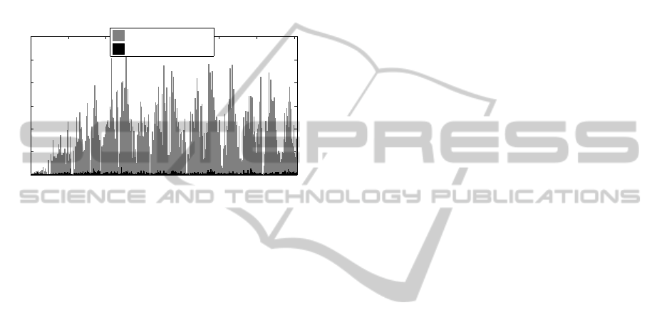
point clouds can be seen in Figure 6. As can be seen

in the ﬁgure, the new distance computations are or-

ders of magnitude faster in the simpliﬁed point cloud

than in the original point cloud.

0 100 200 300 400 500 600 700

0.5

1.5

2.5

Distance computation

Time to compute distance (s)

1 billion points

200 million points

Figure 6: Time for distance computations for the original

and the simpliﬁed point clouds.

6 CONCLUSIONS

It has been veriﬁed that an in-core PQP implementa-

tion can be used even for massive point clouds by di-

viding the point cloud into subsets and then use The-

orem 2 in order to rule out many of the subsets. The-

orem 2 was able to rule out 96% of the subsets so

that only a few subsets had to be considered for each

distance computation. Theorem 2 has a drawback of

not being precise in some cases and therefore forc-

ing reads of subsets that are far away from the object.

This could be avoided by using a fast distance approx-

imation scheme based on the bounding boxes of the

subsets or the extreme points of the convex hulls in

order to approximate how close subsets actually are

before considering all the points. This is appealing

since reading the subset from the hard-disk is the ma-

jor bottleneck in the proposed approach which is why

it is of interest to use a few points to approximate the

distance to the rest of the points.

By simplifying the point cloud using either the

grid-based partitioning or the k-means clustering

method, a simpliﬁed point cloud was created that was

easier to work with. It was seen in Section 5 that

a point cloud with 1 billion points could be simpli-

ﬁed, with ε = 2 cm, to a point cloud with 200 million

points to which the distances could be computed in-

core given 8 GB of memory and therefore decrease

the computation time from 500s to 22s. By allow-

ing the computed shortest distance to deviate by ε, it

is therefore possible to decrease the time for distance

computations signiﬁcantly. It was also seen that the k-

means method provides a simpliﬁed point cloud with

a smaller |P

| than the grid-based partitioning, even

though it is signiﬁcantly slower.

Because methods used to carry out collision de-

tection with massive models are inappropriate for dis-

tance queries, (Yoon et al., 2004), this work ﬁlls a

gap in the literature for distance computations in mas-

sive point clouds. Although methods exist for colli-

sion detection in point clouds, (Pan et al., 2011), their

extension to massive point clouds is not clear. In ad-

dition, given the minimum distance restrictions often

required during path planning, using collision detec-

tion does not seem to be natural. Hence, we have

shown that the path-planning problem requiring min-

imum distances can be solved directly via distance

computations.

Although the method has been shown to be fast,

distance computations are in general slower than

identical collision queries. Hence, if the user’s goal

is simply the fastest computations possible and he or

she does not require the extra distance information,

then it might be beneﬁcial to use a collision based ap-

proach.

In future work we would like to address the fol-

lowing promising avenues for research:

• Use the extreme points of the convex hull of each

subset in order to approximate the distance to the

object when Theorem 2 fails to rule out a subset.

• Take the direction of motion of S into account in

Theorem 2.

• Use bounding boxes instead of swept sphere vol-

umes in PQP in order to decrease the memory re-

quirement for a PQP model.

• Investigate how to choose T optimally as a func-

tion of amount of RAM, |P| and the properties of

the disk(s) used.

ACKNOWLEDGEMENTS

This work was carried out at the Wingquist Labora-

tory VINN Excellence Centre, and is part of the Sus-

tainable Production Initiativeand the Production Area

of Advance at Chalmers University of Technology. It

was supported by the Swedish Governmental Agency

for Innovation Systems.

ApproximateDistanceQueriesforPath-planninginMassivePointClouds

REFERENCES

Berlin, R. (2002). Accurate robot and workcell simulation

based on 3d laser scanning. In Proceedings of the 33rd

ISR (International Symposium on Robotics).

Bialkowski, J., Karaman, S., Otte, M., and Frazzoli, E.

(2013). Efﬁcient collision checking in sampling-

based motion planning. In Algorithmic Foundations

of Robotics X, pages 365–380. Springer.

Carlson, J. S., Spensieri, D., S¨oderberg, R., Bohlin, R., and

Lindkvist, L. (2013). Non-nominal path planning for

robust robotic assembly. Journal of manufacturing

systems, 32(3):429–435.

Dementiev, R., Kettner, L., and Sanders, P. (2008). Stxxl:

standard template library for xxl data sets. Software:

Practice and Experience, 38(6):589–637.

Dupuis, E., Rekleitis, I., Bedwani, J.-L., Lamarche, T., Al-

lard, P., and Zhu, W.-H. (2008). Over-the-horizon

autonomous rover navigation: experimental results.

In International Symposium on Artiﬁcial Intelligence,

Robotics and Automation in Space (i-SAIRAS), Los

Angeles, CA.

Eriksson, D. (2014). Point cloud simpliﬁcation and pro-

cessing for path-planning. Master’s thesis, Chalmers

University of Technology.

Fr¨ohlich, C. and Mettenleiter, M. (2004). Terrestrial laser

scanning—new perspectives in 3d surveying. Interna-

tional Archives of Photogrammetry, Remote Sensing

and Spatial Information Sciences, 36(Part 8):W2.

Hermansson, T., Bohlin, R., Carlson, J. S., and S¨oderberg,

R. (2012). Automatic path planning for wiring harness

installations (wt). In 4th CIRP Conference on Assem-

bly Technology and Systems-CATS 2012, University of

Michigan, Ann Arbor, USA on May 21-23, 2012.

Landa, Y. (2008). Visibility of point clouds and exploratory

path planning in unknown environments. ProQuest.

Landa, Y., Galkowski, D., Huang, Y. R., Joshi, A., Lee,

C., Leung, K. K., Malla, G., Treanor, J., Voroninski,

V., Bertozzi, A. L., et al. (2007). Robotic path plan-

ning and visibility with limited sensor data. In Ameri-

can Control Conference, 2007. ACC’07, pages 5425–

5430. IEEE.

Larsen, E., Gottschalk, S., Lin, M. C., and Manocha, D.

(1999). Fast proximity queries with swept sphere vol-

umes. Technical report, Technical Report TR99-018,

Department of Computer Science, University of North

Carolina.

Latombe, J.-C. (1990). ROBOT MOTION PLANNING.:

Edition en anglais. Springer.

Lauterbach, C., Mo, Q., and Manocha, D. (2010). gprox-

imity: Hierarchical gpu-based operations for collision

and distance queries. In Computer Graphics Forum,

volume 29, pages 419–428. Wiley Online Library.

LaValle, S. M. (2006). Planning algorithms. Cambridge

university press.

Lloyd, S. (1982). Least squares quantization in pcm. In-

formation Theory, IEEE Transactions on, 28(2):129–

137.

Pan, J., Chitta, S., and Manocha, D. (2011). Probabilistic

collision detection between noisy point clouds using

robust classiﬁcation. In International Symposium on

Robotics Research.

Pauly, M., Gross, M., and Kobbelt, L. P. (2002). Efﬁcient

simpliﬁcation of point-sampled surfaces. In Visualiza-

tion, 2002. VIS 2002. IEEE, pages 163–170. IEEE.

Sankaranarayanan, J., Samet, H., and Varshney, A. (2007).

A fast all nearest neighbor algorithm for applications

involving large point-clouds. Computers & Graphics,

31(2):157–174.

Spensieri, D., Bohlin, R., and Carlson, J. S. (2013). Coordi-

nation of robot paths for cycle time minimization. In

CASE, pages 522–527.

Spensieri, D., Carlson, J. S., Bohlin, R., and S¨oderberg, R.

(2008). Integrating assembly design, sequence opti-

mization, and advanced path planning. ASME Confer-

ence Proceedings, (43253):73–81.

Sucan, I. A., Kalakrishnan, M., and Chitta, S. (2010).

Combining planning techniques for manipulation us-

ing realtime perception. In Robotics and Automa-

tion (ICRA), 2010 IEEE International Conference on,

pages 2895–2901. IEEE.

Tafuri, S., Shellshear, E., Bohlin, R., and Carlson, J. S.

(2012). Automatic collision free path planning in hy-

brid triangle and point models: a case study. In Pro-

ceedings of the Winter Simulation Conference, page

282. Winter Simulation Conference.

Volvo (2013). Volvo Cars in Gothenburg, Personal commu-

nication.

Yoon, S.-E., Salomon, B., Lin, M., and Manocha, D. (2004).

Fast collision detection between massive models us-

ing dynamic simpliﬁcation. In Proceedings of the

2004 Eurographics/ACM SIGGRAPH symposium on

Geometry processing, pages 136–146. ACM.

ICINCO2014-11thInternationalConferenceonInformaticsinControl,AutomationandRobotics