
Complexity of Rule Sets Induced from Incomplete Data with
Attribute-concept Values and “Do Not Care” Conditions
Patrick G. Clark
1
and Jerzy W. Grzymala-Busse
1,2
1
Department of Electrical Engineering and Computer Science, University of Kansas, Lawrence, KS 66045, U.S.A.
2
Department of Expert Systems and Artificial Intelligence, University of Information Technology and Management,
35-225 Rzeszow, Poland
Keywords:
Data Mining, Rough Set Theory, Probabilistic Approximations, MLEM2 Rule Induction Algorithm,
Attribute-concept Values, “Do Not Care” Conditions.
Abstract:
In this paper we study the complexity of rule sets induced from incomplete data sets with two interpretations
of missing attribute values: attribute-concept values and “do not care” conditions. Experiments are conducted
on 176 data sets, using three kinds of probabilistic approximations (lower, middle and upper) and the MLEM2
rule induction system. The goal of our research is to determine the interpretation and approximation that
produces the least complex rule sets. In our experiment results, the size of the rule set is smaller for attribute-
concept values for 12 combinations of the type of data set and approximation, for one combination the size
of the rule sets is smaller for “do not care” conditions and for the remaining 11 combinations the difference
in performance is statistically insignificant (5% significance level). The total number of conditions is smaller
for attribute-concept values for ten combinations, for two combinations the total number of conditions is
smaller for “do not care” conditions, while for the remaining 12 combinations the difference in performance
is statistically insignificant. Thus, we may claim that attribute-concept values are better than “do not care”
conditions in terms of rule complexity.
1 INTRODUCTION
Rough set theory has been applied to many areas
of data mining. Fundamental concepts of rough set
theory are standard lower and upper approximations.
In this paper we will use probabilistic approxima-
tions. A probabilistic approximation, associated with
a probability α, is a generalization of the standard ap-
proximation. For α = 1, the probabilistic approxima-
tion is reduced to the lower approximation; for very
small positive α, it is reduced to the upper approxi-
mation. Research on theoretical properties of prob-
abilistic approximations started from (Pawlak et al.,
1988) and then continued in many papers, see, e.g.,
(Pawlak and Skowron, 2007; Pawlak et al., 1988;
´
Sle¸zak and Ziarko, 2005; Yao, 2008; Yao and Wong,
1992; Ziarko, 2008).
Incomplete data sets may be analyzed using global
approximations such as singleton, subset and concept
(Grzymala-Busse, 2003; Grzymala-Busse, 2004a;
Grzymala-Busse, 2004b). Probabilistic approxima-
tions for incomplete data sets and based on an arbi-
trary binary relation were introduced in (Grzymala-
Busse, 2011). The first experimental results using
probabilistic approximations were published in (Clark
and Grzymala-Busse, 2011).
For our experiments we use 176 incomplete data
sets, with two types of missing attribute values:
attribute-concept values (Grzymala-Busse, 2004c)
and “do not care” conditions (Grzymala-Busse, 1991;
Kryszkiewicz, 1995; Stefanowski and Tsoukias,
1999). Additionally, in our experiments we use three
types of approximations: lower, middle, and upper.
The middle approximation is the most typical proba-
bilistic approximation, with α = 0.5.
In (Clark and Grzymala-Busse, 2014), the results
indicate that rule set performance, in terms of error
rate, for both missing attribute value interpretations
is not significantly different. As a result, given two
rule sets with the same error rate, the more desirable
would be the least complex, both for comprehension
and computation performance. Therefore, the main
objective of this paper is research on the complex-
ity of rule sets induced from data sets with attribute-
concept values and “do not care” conditions. Com-
plexity is defined in terms of the number of rules
56
Clark P. and Grzymala-Busse J..
Complexity of Rule Sets Induced from Incomplete Data with Attribute-concept Values and "Do Not Care" Conditions.
DOI: 10.5220/0005003400560063
In Proceedings of 3rd International Conference on Data Management Technologies and Applications (DATA-2014), pages 56-63
ISBN: 978-989-758-035-2
Copyright
c
2014 SCITEPRESS (Science and Technology Publications, Lda.)

and the number of rule conditions, with larger num-
bers indicating greater complexity. Our main result is
that the simpler rule sets are induced from data sets
in which missing attribute values are interpreted as
attribute-concept values.
Our secondary objective is to identify the approx-
imation (lower, middle or upper) that produces the
lowest rule complexity. Our conclusion is that all
three kinds of approximations do not differ signifi-
cantly with respect to the complexity of induced rule
sets.
2 INCOMPLETE DATA
We assume that the input data sets are presented in
the form of a decision table. An example of a deci-
sion table is shown in Table 1. Rows of the decision
table represent cases, while columns are labeled by
variables. The set of all cases will be denoted by U.
In Table 1, U = {1, 2, 3, 4, 5, 6, 7, 8}. Independent
variables are called attributes and a dependent vari-
able is called a decision and is denoted by d. The set
of all attributes will be denoted by A. In Table 1, A =
{Education, Skills, Experience}. The value for a case
x and an attribute a will be denoted by a(x).
In this paper we distinguish between two interpre-
tations of missing attribute values: attribute-concept
values and “do not care” conditions. Attribute-
concept values, denoted by “−”, indicate that the
missing attribute value may be replaced by any speci-
fied attribute value for a given concept. For example,
if a patient is sick with flu, and if for other such pa-
tients the value of temperature is high or very-high,
then we will replace the missing attribute values of
temperature by values high and very-high, for details
see (Grzymala-Busse, 2004c). “Do not care” con-
ditions , denoted by “*”, mean that the original at-
tribute values are irrelevant, so we may replace them
by any attribute value, for details see (Grzymala-
Busse, 1991; Kryszkiewicz, 1995; Stefanowski and
Tsoukias, 1999). Table 1 presents an incomplete data
set affected by both attribute-concept values and “do
not care” conditions.
One of the most important ideas of rough set the-
ory (Pawlak, 1982) is an indiscernibility relation, de-
fined for complete data sets. Let B be a nonempty
subset of A. The indiscernibility relation R(B) is a re-
lation on U defined for x, y ∈ U as follows:
(x, y) ∈ R(B) if and only if ∀a ∈ B (a(x) = a(y)).
The indiscernibility relation R(B) is an equivalence
relation. Equivalence classes of R(B) are called ele-
mentary sets of B and are denoted by [x]
B
. A subset of
Table 1: A decision table.
Attributes Decision
Case Education Skills Experience Productivity
1 higher high − high
2 * high low high
3 secondary − high high
4 higher * high high
5 elementary high low low
6 secondary − high low
7 − low high low
8 elementary * − low
U is called B-definable if it is a union of elementary
sets of B.
The set X of all cases defined by the same value
of the decision d is called a concept. For example,
a concept associated with the value low of the deci-
sion Productivity is the set {1, 2, 3, 4}. The largest
B-definable set contained in X is called the B-lower
approximation of X , denoted by appr
B
(X), and de-
fined as follows
∪{[x]
B
| [x]
B
⊆ X },
while the smallest B-definable set containing X , de-
noted by appr
B
(X) is called the B-upper approxima-
tion of X, and is defined as follows
∪{[x]
B
| [x ]
B
∩ X ̸=
/
0}.
For a variable a and its value v, (a, v) is called
a variable-value pair. A block of (a, v), denoted by
[(a, v)], is the set {x ∈ U | a(x) = v} (Grzymala-Busse,
1992).
For incomplete decision tables the definition of a
block of an attribute-value pair is modified in the fol-
lowing way.
• If for an attribute a there exists a case x such that
a(x) = −, then the corresponding case x should be
included in blocks [(a, v)] for all specified values
v ∈ V (x, a) of attribute a, where
V (x, a) =
= {a(y) | a(y) is specified, y ∈ U, d(y) = d(x )},
• If for an attribute a there exists a case x such that
a(x) = ∗, then the case x should be included in
blocks [(a, v)] for all specified values v of the at-
tribute a.
For the data set from Table 1, V (1, Experience) =
{low, high}, V (3, Skills) = {high},
ComplexityofRuleSetsInducedfromIncompleteDatawithAttribute-conceptValuesand"DoNotCare"Conditions
57

V (6, Skills) = {low, high}, V (7, Education) =
{elementary, secondary} and V (8, Experience) =
{low, high}.
For the data set from Table 1 the blocks of
attribute-value pairs are:
[(Education, elementary)] = {2, 5, 7, 8},
[(Education, secondary)] = {2, 3, 6, 7},
[(Education, higher)] = {1, 2, 4},
[(Skills, low)] = {4, 6, 7, 8},
[(Skills, high)] = {1, 2, 3, 4, 5, 6, 8},
[(Experience, low)] = {1, 2, 5, 8},
[(Experience, high)] = {1, 3, 4, 6, 7, 8}.
For a case x ∈ U and B ⊆ A, the characteristic set
K
B
(x) is defined as the intersection of the sets K(x, a),
for all a ∈ B, where the set K(x, a) is defined in the
following way:
• If a(x) is specified, then K(x, a) is the block
[(a, a(x))] of attribute a and its value a(x),
• If a(x) = −, then the corresponding set K(x, a)
is equal to the union of all blocks of attribute-
value pairs (a, v), where v ∈ V (x, a) if V (x, a) is
nonempty. If V (x, a) is empty, K(x, a) = U,
• If a(x) = ∗ then the set K(x, a) = U, where U is
the set of all cases.
For Table 1 and B = A,
K
A
(1) = {1, 2, 4},
K
A
(2) = {1, 2, 5, 8},
K
A
(3) = {3, 6},
K
A
(4) = {1, 4},
K
A
(5) = {2, 5, 8},
K
A
(6) = {3, 6, 7},
K
A
(7) = {6, 7, 8},
K
A
(8) = {2, 5, 7, 8}.
Note that for incomplete data there are a few
possible ways to define approximations (Grzymala-
Busse, 2003), we used concept approximations
(Grzymala-Busse, 2011) since our previous experi-
ments indicated that such approximations are most ef-
ficient (Grzymala-Busse, 2011). A B-concept lower
approximation of the concept X is defined as follows:
BX = ∪{K
B
(x) | x ∈ X, K
B
(x) ⊆ X },
while a B-concept upper approximation of the con-
cept X is defined by:
BX = ∪{K
B
(x) | x ∈ X, K
B
(x) ∩ X ̸=
/
0} =
= ∪{K
B
(x) | x ∈ X}.
For Table 1, A-concept lower and A-concept upper
approximations of the concept {5, 6, 7, 8} are:
A{5, 6, 7, 8} = {6, 7, 8},
A{5, 6, 7, 8} = {2, 3, 5, 6, 7, 8}.
3 PROBABILISTIC
APPROXIMATIONS
For completely specified data sets a probabilistic ap-
proximation is defined as follows
appr
α
(X) = ∪{[x] | x ∈ U, P(X | [x]) ≥ α},
α is a parameter, 0 < α ≤ 1, see (Grzymala-Busse,
2011; Grzymala-Busse and Ziarko, 2003; Pawlak
et al., 1988; Wong and Ziarko, 1986; Yao, 2008;
Ziarko, 1993). Additionally, for simplicity, the ele-
mentary sets [x]
A
are denoted by [x]. For discussion
on how this definition is related to the variable preci-
sion asymmetric rough sets see (Clark and Grzymala-
Busse, 2011; Grzymala-Busse, 2011).
Note that if α = 1, the probabilistic approximation
becomes the standard lower approximation and if α is
small, close to 0, in our experiments it is 0.001, the
same definition describes the standard upper approxi-
mation.
For incomplete data sets, a B-concept probabilis-
tic approximation is defined by the following formula
(Grzymala-Busse, 2011)
∪{K
B
(x) | x ∈ X, Pr(X|K
B
(x)) ≥ α}.
For simplicity, we will denote K
A
(x) by K(x)
and the A-concept probabilistic approximation will be
called a probabilistic approximation.
For Table 1 and the concept X = [(Productivity,
low)] = {5, 6, 7, 8}, there exist three distinct three
distinct probabilistic approximations:
appr
1.0
(
{
5
,
6
,
7
,
8
}
) =
{
6
,
7
,
8
}
,
appr
0.75
({5, 6, 7, 8}) = {2, 5, 6, 7, 8},
and
appr
0.001
({5, 6, 7, 8}) = {2, 3, 5, 6, 7, 8}.
The special probabilistic approximations with the
parameter α = 0.5 will be called a middle approxima-
tion.
4 EXPERIMENTS
Our experiments are based on eight data sets available
from the University of California at Irvine Machine
Learning Repository, see Table 2.
For every data set a set of templates is created
by incrementally replacing a percentage of existing
specified attribute values (at a 5% increment) with
attribute-concept values. Thus, we started each se-
ries of experiments with no attribute-concept values,
DATA2014-3rdInternationalConferenceonDataManagementTechnologiesandApplications
58
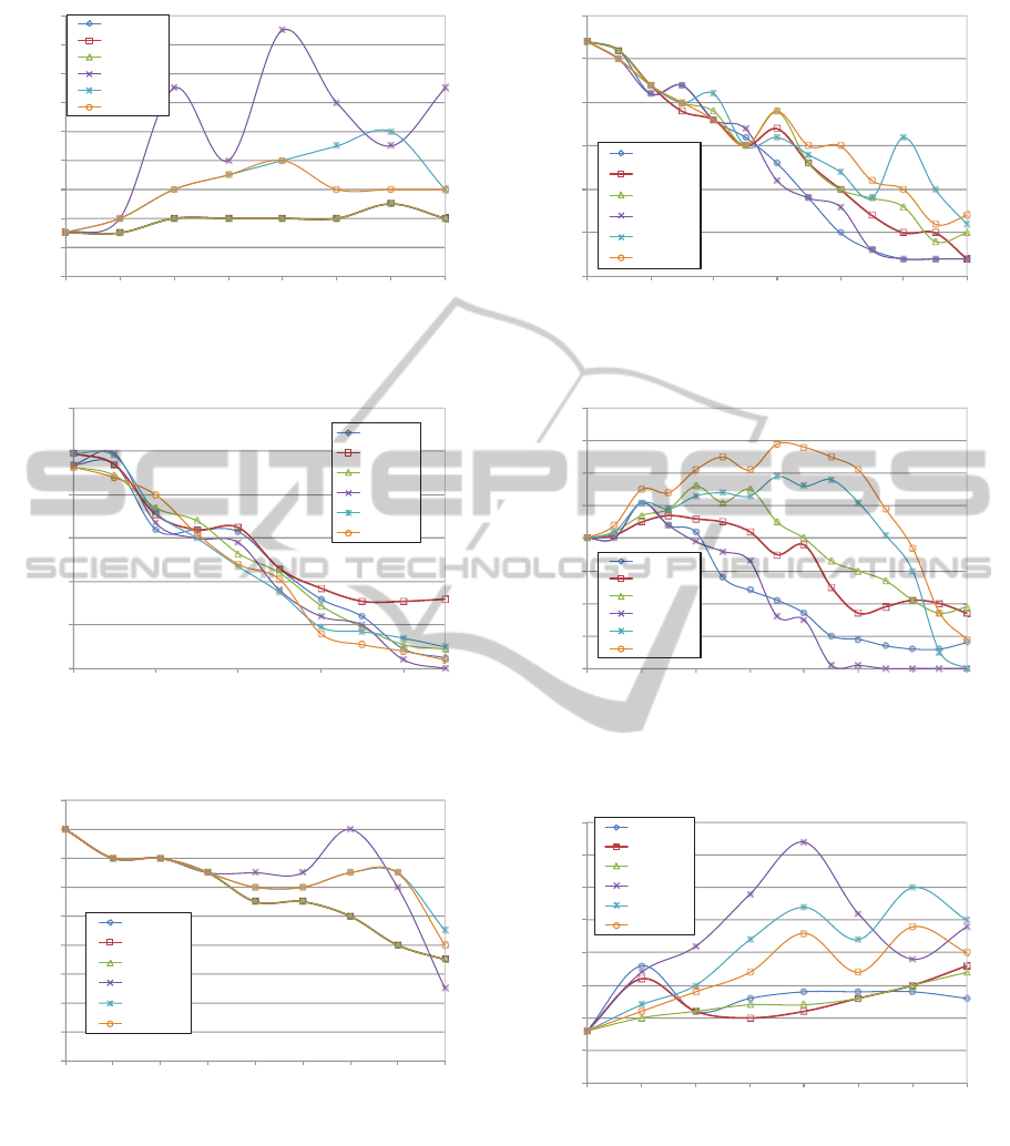
0
2
4
6
8
10
12
14
16
18
0 5 10 15 20 25 30
35
Rule count
Missing attributes (%)
Lower, -
Middle, -
Upper, -
Lower, *
Middle, *
Upper, *
Figure 1: Size of the rule set for the Bankruptcy data set.
0
20
40
60
80
100
120
0 10 20 30 40
Rule count
Missing attributes (%)
Lower, -
Middle, -
Upper, -
Lower, *
Middle, *
Upper, *
Figure 2: Size of the rule set for the Breast cancer data set.
0
2
4
6
8
10
12
14
16
18
0 5 10 15 20 25 30 35
40
Rule count
Missing attributes (%)
Lower, -
Middle, -
Upper, -
Lower, *
Middle, *
Upper, *
Figure 3: Size of the rule set for the Echocardiogram data
set.
then we changed 5% of specified values to attribute-
concept values, then we changed an additional 5% of
specified values to attribute-concept values, etc., un-
til at least one entire row of the data set is full of
attribute-concept values. Then three attempts were
made to change the configuration of new attribute-
concept values and either a new data set with an extra
5% of attribute-concept is created or the process is
0
5
10
15
20
25
30
0 10 20 30 40 50
60
Rule count
Missing attributes (%)
Lower, -
Middle, -
Upper, -
Lower, *
Middle, *
Upper, *
Figure 4: Size of the rule set for the Hepatitis data set.
0
10
20
30
40
50
60
70
80
0 10 20 30 40 50 60 70
Rule count
Missing attributes (%)
Lower, -
Middle, -
Upper, -
Lower, *
Middle, *
Upper, *
Figure 5: Size of the rule set for the Image segmentation
data set.
0
5
10
15
20
25
30
35
40
0 5 10 15 20 25 30 35
Rule count
Missing attributes (%)
Lower, -
Middle, -
Upper, -
Lower, *
Middle, *
Upper, *
Figure 6: Size of the rule set for the Iris data set.
terminated. Additionally, the same formed templates
are edited for further experiments by replacing each “-
”, representing attribute-concept values with “*”, rep-
resenting “do not care” conditions.
For any data set there is some maximum for the
percentage of missing attribute values. For example,
for the bankruptcy data set, it is 35%. Hence, for the
bankruptcy data set, there exist seven data sets with
ComplexityofRuleSetsInducedfromIncompleteDatawithAttribute-conceptValuesand"DoNotCare"Conditions
59
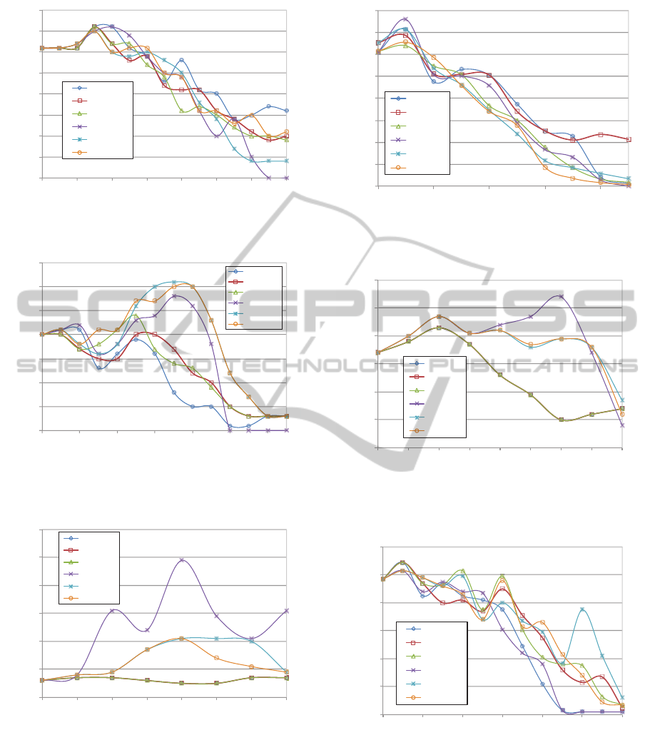
0
5
10
15
20
25
30
35
40
0 10 20 30 40 50 60 70
Rule count
Missing attributes (%)
Lower, -
Middle, -
Upper, -
Lower, *
Middle, *
Upper, *
Figure 7: Size of the rule set for the Lymphography data set.
0
5
10
15
20
25
30
35
0 10 20 30 40 50 60
Rule count
Missing attributes (%)
Lower, -
Middle, -
Upper, -
Lower, *
Middle, *
Upper, *
Figure 8: Size of the rule set for the Wine recognition data
set.
0
10
20
30
40
50
60
0 5 10 15 20 25 30
35
Condition count
Missing attributes (%)
Lower, -
Middle, -
Upper, -
Lower, *
Middle, *
Upper, *
Figure 9: Number of conditions for the Bankruptcy data set.
attribute-concept values and seven data sets with “do
not care” conditions, for a total of 15 data sets (the ad-
ditional data set is complete, with no missing attribute
values). In a similar process for the breast cancer,
echocardiogram, hepatitis, image segmentation, iris,
lymphography and wine recognition data sets we cre-
ated 19, 17, 25, 29, 15, 29, and 27 data sets. Hence
the total number of data sets is 176.
0
50
100
150
200
250
300
350
400
0 10 20 30 40
Condition count
Missing attributes (%)
Lower, -
Middle, -
Upper, -
Lower, *
Middle, *
Upper, *
Figure 10: Number of conditions for the Breast cancer data
set.
0
10
20
30
40
50
60
0 5 10 15 20 25 30 35
40
Condition count
Missing attributes (%)
Lower, -
Middle, -
Upper, -
Lower, *
Middle, *
Upper, *
Figure 11: Number of conditions for the Echocardiogram
data set.
0
20
40
60
80
100
120
0 10 20 30 40 50
60
Condition count
Missing attributes (%)
Lower, -
Middle, -
Upper, -
Lower, *
Middle, *
Upper, *
Figure 12: Number of conditions for the Hepatitis data set.
Results of our experiments are presented in Fig-
ures 1–16.
DATA2014-3rdInternationalConferenceonDataManagementTechnologiesandApplications
60
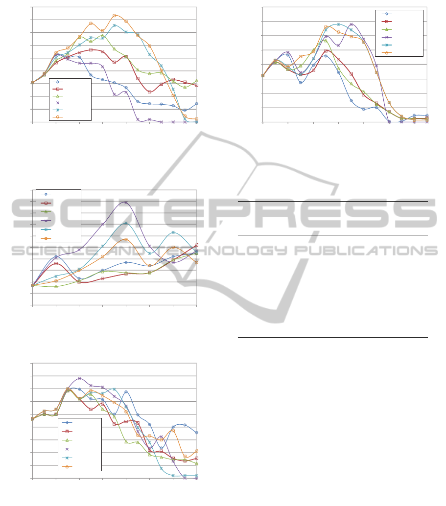
0
50
100
150
200
250
300
350
400
450
0 10 20 30 40 50 60
70
Condition count
Missing attributes (%)
Lower, -
Middle, -
Upper, -
Lower, *
Middle, *
Upper, *
Figure 13: Number of conditions for the Image segmenta-
tion data set.
0
10
20
30
40
50
60
70
80
90
100
0 5 10 15 20 25 30
35
Condition count
Missing attributes (%)
Lower, -
Middle, -
Upper, -
Lower, *
Middle, *
Upper, *
Figure 14: Number of conditions for the Iris data set.
0
20
40
60
80
100
120
140
160
180
0 10 20 30 40 50 60
70
Condition count
Missing attributes (%)
Lower, -
Middle, -
Upper, -
Lower, *
Middle, *
Upper, *
Figure 15: Number of conditions for the Lymphography
data set.
5 DISCUSSION
First we compare two interpretations of missing at-
tribute values, attribute-concept values and “do not
care” conditions with respect to the rule set size. For
0
20
40
60
80
100
120
140
160
0 10 20 30 40 50 60
Condition count
Missing attributes (%)
Lower, -
Middle, -
Upper, -
Lower, *
Middle, *
Upper, *
Figure 16: Number of conditions for the Wine recognition
data set.
Table 2: Data sets used for experiments.
Data set Number of
cases attributes concepts
Bankruptcy 66 5 2
Breast cancer 277 9 2
Echocardiogram 74 7 2
Hepatitis 155 19 2
Image segmentation 210 19 7
Iris 150 4 3
Lymphography 148 18 4
Wine recognition 178 13 3
every data set type, separately for lower, middle and
upper approximations, the Wilcoxon matched-pairs
signed rank test is used with a 5% level of significance
two-tailed test. With eight data set types and three ap-
proximation types, the total number of combinations
is 24.
For 12 combinations the rule set size is smaller for
attribute-concept values: bankruptcy data set with all
three types of approximations, hepatitis data set with
middle and upper approximations, image segmenta-
tion data set with middle and upper approximations,
iris data set with all three types of approximations
and wine recognition data set with middle and upper
approximations. For one combination, breast cancer
data set with middle approximations, the size of the
rule set is smaller for “do not care” conditions. For
the remaining 11 combinations, the difference in the
rule set size between attribute-concept values and “do
not care” conditions is insignificant. Therefore there
is strong evidence that attribute-concept values pro-
vide for smaller rule set sizes than “do not care” con-
ditions.
Similarly, for the total number of conditions in a
rule set, in ten combinations this number is smaller for
ComplexityofRuleSetsInducedfromIncompleteDatawithAttribute-conceptValuesand"DoNotCare"Conditions
61

attribute-concept values: bankruptcy data set with all
three types of approximations, echocardiogram data
set with all three types of approximations, lymphog-
raphy data set with upper approximations and wine
recognition data set with all three types of approx-
imations. For two combinations the total number
of conditions in the rule set is smaller for “do not
care” conditions: breast cancer data set with middle
approximations and image recognition data set with
lower approximations. For the remaining 12 combi-
nations the difference in the total number of condi-
tions in rule sets between attribute-concept values and
“do not care” conditions is insignificant. Thus there
is evidence that attribute-concept values provide for
a smaller total number of conditions in rule sets than
“do not care” conditions.
Next, for a given interpretation of missing at-
tribute values we compare all three types of approx-
imations in terms of the rule set size and the total
number of conditions in the rule set. For all eight
types of data sets, we compare lower approximations
with middle and upper approximations, and middle
approximations with upper approximations. This ex-
periment setup results in a total of 24 combinations
and the Friedman Rank Sums test, with 5% signifi-
cance level, is used.
The rule set size is smaller for lower approxi-
mations than for upper approximations in four com-
binations of the type of data set and type of miss-
ing attribute value: hepatitis data set with attribute-
concept values, image segmentation data set with both
attribute-concept values and “do not care” conditions
and wine recognition data set with “do not care” con-
ditions. The rule set size is smaller for lower approx-
imations than for middle approximations for three
combinations of the data set type and missing attribute
value type: image segmentation data set with both
attribute-concept values and “do not care” conditions
and hepatitis data set with attribute-concept values.
The rule set size is smaller for upper approximations
than for lower approximations in three combinations:
bankruptcy data set with “do not care” conditions, iris
data set with “do not care” conditions and lymphog-
raphy data set with attribute-concept values. Finally,
the rule set size is smaller for upper approximations
than for middle approximations in one combination:
breast cancer data set with attribute-concept values.
In the remaining 13 combinations the difference be-
tween all three approximations is insignificant. There
is weak evidence that lower approximations might be
better than the remaining approximations.
The total number of conditions in a rule set is
smaller for lower approximations than for upper ap-
proximations in three combinations of data set type
and missing attribute value type: hepatitis data set
with attribute-concept values and image segmentation
data set with both attribute-concept values and “do
not care” conditions. The total number of conditions
in a rule set is smaller for lower approximations than
for middle approximations in one combination: image
segmentation data set with “do not care” conditions.
The total number of conditions in a rule set is smaller
for middle approximations than for lower approxima-
tions in one combination: lymphography data set with
attribute-concept values. The total number of condi-
tions in a rule set is smaller for upper approximations
than for lower approximations in three combinations:
bankruptcy data set with “do not care” conditions, iris
data set with “do not care” conditions and lymphogra-
phy
data set with attribute-concept values. Finally, the
total number of conditions in a rule set is smaller for
upper approximations than for middle approximations
in one combination: lymphography data set with the
attribute-concept values. In the remaining 15 combi-
nations the difference between all three approxima-
tions is insignificant. Practically speaking, we do not
have enough evidence to tell which approximation is
the best.
6 RELATED WORK
Rough set concepts and the indiscernibility relation
are introduced in (Pawlak, 1982) with additional re-
search explaining theoretical concepts of probabilistic
approximations in (Pawlak et al., 1988). Further re-
search was conducted in the area of probabilistic types
of approximations in other efforts, comparing them
to deterministic approaches and studying other exten-
sions in (Pawlak and Skowron, 2007; Pawlak et al.,
1988;
´
Sle¸zak and Ziarko, 2005; Yao, 2008; Yao and
Wong, 1992; Ziarko, 2008).
In (Grzymala-Busse, 2003; Grzymala-Busse,
2004a; Grzymala-Busse, 2004b), three global approx-
imations are defined: singleton, subset and concept.
The papers also include a study of these approxima-
tions with incomplete data. In our work, concept ap-
proximations are used in conjunction with probabilis-
tic approximations on incomplete data sets. These
concepts were introduced in (Grzymala-Busse, 2011)
and include definitions of B-concept probabilistic ap-
proximations with discussions on how the definition
is related to variable precision asymmetric rough sets.
In addition, the first experimental results are studied
in (Clark and Grzymala-Busse, 2011).
DATA2014-3rdInternationalConferenceonDataManagementTechnologiesandApplications
62

7 CONCLUSIONS
As follows from our experiments, there is evidence
that the rule set size is smaller for the attribute-
concept interpretation of missing attribute values than
for the “do not care” condition interpretation. The to-
tal number of conditions in rule sets is also smaller for
attribute-concept interpretation of missing attribute
values. Thus we may claim attribute-concept values
are better than “do not care” conditions as an inter-
pretation of a missing attribute value in terms of rule
complexity.
Furthermore, all three kinds of approximations
(lower, middle and upper) do not differ significantly
with respect to the complexity of induced rule sets.
Future direction this work might take is an inves-
tigation of other interpretations of missing attribute
values and a comparison of the complexity of the rule
sets produced.
REFERENCES
Clark, P. G. and Grzymala-Busse, J. W. (2011). Experi-
ments on probabilistic approximations. In Proceed-
ings of the 2011 IEEE International Conference on
Granular Computing, pages 144–149.
Clark, P. G. and Grzymala-Busse, J. W. (2014). Mining in-
complete data with attribute-concept values and “do
not care” conditions. In Proceedings of the 9th Inter-
national Conference on Hybrid Artificial Intelligence
Systems, pages 146–167.
Grzymala-Busse, J. W. (1991). On the unknown attribute
values in learning from examples. In Proceedings
of the ISMIS-91, 6th International Symposium on
Methodologies for Intelligent Systems, pages 368–
377.
Grzymala-Busse, J. W. (1992). LERS—a system for learn-
ing from examples based on rough sets. In Slowinski,
R., editor, Intelligent Decision Support. Handbook of
Applications and Advances of the Rough Set Theory,
pages 3–18. Kluwer Academic Publishers, Dordrecht,
Boston, London.
Grzymala-Busse, J. W. (2003). Rough set strategies to data
with missing attribute values. In Workshop Notes,
Foundations and New Directions of Data Mining, in
conjunction with the 3-rd International Conference on
Data Mining, pages 56–63.
Grzymala-Busse, J. W. (2004a). Characteristic relations for
incomplete data: A generalization of the indiscerni-
bility relation. In Proceedings of the Fourth Interna-
tional Conference on Rough Sets and Current Trends
in Computing, pages 244–253.
Grzymala-Busse, J. W. (2004b). Data with missing attribute
values: Generalization of indiscernibility relation and
rule induction. Transactions on Rough Sets, 1:78–95.
Grzymala-Busse, J. W. (2004c). Three approaches to miss-
ing attribute values—a rough set perspective. In Pro-
ceedings of the Workshop on Foundation of Data Min-
ing, in conjunction with the Fourth IEEE International
Conference on Data Mining, pages 55–62.
Grzymala-Busse, J. W. (2011). Generalized parameterized
approximations. In Proceedings of the RSKT 2011,
the 6-th International Conference on Rough Sets and
Knowledge Technology, pages 136–145.
Grzymala-Busse, J. W. and Ziarko, W. (2003). Data mining
based on rough sets. In Wang, J., editor, Data Mining:
Opportunities and Challenges, pages 142–173. Idea
Group Publ., Hershey, PA.
Kryszkiewicz, M. (1995). Rough set approach to incom-
plete information systems. In Proceedings of the
Second Annual Joint Conference on Information Sci-
ences, pages 194–197.
Pawlak, Z. (1982). Rough sets. International Journal of
Computer and Information Sciences, 11:341–356.
Pawlak, Z. and Skowron, A. (2007). Rough sets: Some
extensions. Information Sciences, 177:28–40.
Pawlak, Z., Wong, S. K. M., and Ziarko, W. (1988). Rough
sets: probabilistic versus deterministic approach. In-
ternational Journal of Man-Machine Studies, 29:81–
95.
´
Sle¸zak, D. and Ziarko, W. (2005). The investigation of the
bayesian rough set model. International Journal of
Approximate Reasoning, 40:81–91.
Stefanowski, J. and Tsoukias, A. (1999). On the exten-
sion of rough sets under incomplete information. In
Proceedings of the RSFDGrC’1999, 7th International
Workshop on New Directions in Rough Sets, Data
Mining, and Granular-Soft Computing, pages 73–81.
Wong, S. K. M. and Ziarko, W. (1986). INFER—an adap-
tive decision support system based on the probabilistic
approximate classification. In Proceedings of the 6-th
International Workshop on Expert Systems and their
Applications, pages 713–726.
Yao, Y. Y. (2008). Probabilistic rough set approxima-
tions. International Journal of Approximate Reason-
ing, 49:255–271.
Yao, Y. Y. and Wong, S. K. M. (1992). A decision theoretic
framework for approximate concepts. International
Journal of Man-Machine Studies, 37:793–809.
Ziarko, W. (1993). Variable precision rough set model.
Journal of Computer and System Sciences, 46(1):39–
59.
Ziarko, W. (2008). Probabilistic approach to rough
sets. International Journal of Approximate Reason-
ing, 49:272–284.
ComplexityofRuleSetsInducedfromIncompleteDatawithAttribute-conceptValuesand"DoNotCare"Conditions
63
