
Adaptive Gauss Hermite Filter for Parameter
and State Estimation of Nonlinear Systems
Aritro Dey, Manasi Das, Smita Sadhu and T. K. Ghoshal
Department of Electrical Engg., Jadavpur University, Kolkata - 700032, India
Keywords: Adaptive Filters, Nonlinear Filtering, Gauss Hermite Quadrature Rule, State Estimation, Parameter
Estimation.
Abstract: This paper presents an adaptive Gauss Hermite filter for nonlinear signal models in the situation when the
measurement noise statistics is unknown. The proposed nonlinear filter, based on the Gauss Hermite
quadrature rule, can ensure satisfactory estimation performance despite the problem of unknown
measurement noise statistics by online adaptation. Results of Monte Carlo Simulation demonstrate the
efficacy of the proposed filter for joint estimation of parameters and states using an object tracking problem.
1 INTRODUCTION
Optimal filtering and estimation require knowledge
about the covariances of process and measurement
noise (Simon, 2006). Estimation performance is
known to deteriorate when such noise covariances
are unknown. One solution to overcome the above
problem is to use adaptive estimators. In this paper,
an yet unreported adaptive sigma point filter has
been proposed for nonlinear systems where the
measurement noise covariance is unknown.
The estimator proposed here is based on the
Gauss Hermite quadrature rule (Ito, 2000;
Arasaratnam, 2007) and belongs to the family of
sigma point filters. Sigma point filters (Lefebvre,
2004) are derivative free filters and had been widely
reported in literature on nonlinear estimation as
these filters overcome the well known shortcomings
of the Extended Kalman Filter (EKF). Despite the
extensive computation effort Gauss Hermite filters
(GHF) stand out in certain situations in comparison
to Unscented Kalman filters (UKF), Central
Difference filter (CDF) (Ito, 2000) and simulation
based filters like Particle filters (Arasaratnam,
2007).
Even this sophisticated filtering algorithm fails
to provide accurate estimation results in the face of
unknown noise covariances as discussed before.
This paper attempts to overcome this limitation
proposing an adaptive Gauss Hermite quadrature
filter which has been developed by incorporating
adaptation steps in the framework of Gauss Hermite
quadrature filter. The adaptation steps in the
proposed filter employ “covariance matching
method” as inspired from the adaptive linear filters
(Mehra, 1972; Maybeck, 1982; Myer, 1976). Like
the cited previous work the proposed method also
makes use of the statistics of ‘innovation’ (defined
as the difference between the a priori estimate of
measurement and the actual measurement) sequence
for adaptation. Unlike (Myer, 1976), in the work of
(Mehra, 1972; Maybeck, 1982) the algorithm has
been made computationally more efficient by
eliminating the need to use previous history of a
priori error covariance.
Adaptive nonlinear filters like adaptive EKF
(Busse, 2003), adaptive UKF (Das, 2013) or other
adaptive derivative free sigma point filters like
adaptive Divided Difference filter (adaptive DDF)
(Karlgaard, 2011) are also reported in the literature.
In general, adaptive filters are categorized into
two classes depending on the adaptation of the
process noise covariance (Q-adaptive filter), or the
measurement noise covariance (R-adaptive filter).
As the present work is based on measurement noise
adaptation (R-adaptation) the literature review
focuses on R adaptive nonlinear filters. The R
adaptive UKF based on innovation sequence by
(Das, 2013) reports direct adaptation of R while R
adaptive UKF by (Hajiyev, 2014) prefers scaling
factor based adaptation, an equally accepted method
of adaptation. A Robust adaptive DDF presented in
(Karlgaard, 2011) emphasizes on robustness in
presence of outliers and also adapts the unknown
583
Dey A., Das M., Sadhu S. and Ghoshal T..
Adaptive Gauss Hermite Filter for Parameter and State Estimation of Nonlinear Systems.
DOI: 10.5220/0005004505830589
In Proceedings of the 11th International Conference on Informatics in Control, Automation and Robotics (ICINCO-2014), pages 583-589
ISBN: 978-989-758-039-0
Copyright
c
2014 SCITEPRESS (Science and Technology Publications, Lda.)

noise covariances using the innovation based Q and
R adaptation.
The proposed filter uses Gauss Hermite
quadrature rule for evaluation of the integrals
encountered in nonlinear Bayesian filtering problem
(Ito, 2000) and also incorporates the steps for R
adaptation. Only the R adaptive version of adaptive
GHF based on innovation sequence is reported here.
The Q adaptive version (addresses the
complementary problem of R adaptation) was
proposed by the present authors in (Dey, 2014) for
joint estimation of states and parameters.
The adaptive GHF, which has not yet been
reported in the recent literature to the best
knowledge of the authors, has the following
advantages:
(i) Like other derivative free filters the proposed
filter replaces computation of Jacobian and Hessian
matrices by some functional evaluations, (ii) It has
been demonstrated in (Ito, 2000) that Gauss Hermite
quadrature filters provide better estimation
performance compared to UKF and CDF for certain
nonlinear systems and such advantages are expected
to be inherited by its adaptive version. It has also
been reported in (Arasaratnam, 2007) that in certain
situations Gauss Hermite quadrature filters can
ensure estimation accuracy comparable to that of
much more computationally intensive simulation
based filters like Particle filters, (iii) Being a direct
quadrature formula, the proposed filter does not
need the discerning choice of tuning parameters like
the UKF.
The proposed filter is evaluated with the help of
two case studies. The case studies which use a
benchmark nonlinear estimation problem and a well
known ballistic object tracking problem demonstrate
that the proposed filter is capable of joint estimation
of parameters and states.
2 ADAPTIVE GAUSS HERMITE
FILTER
2.1 Problem Statement
We consider nonlinear dynamic equations of a
system as given below
kkk
xfx
1
(1)
kkk
xgy
(2)
where
n
k
Rx is a state vector,
m
k
Ry is
output vector. The zero mean process and
measurement noises (assumed Gaussian) are denoted
as
QR
n
k
,0~
,
k
m
k
RR ,0~
.The process
noise covariance is a known constant matrix.
However, the measurement noise covariance being
unknown it is to be adapted at every time instants.
2.2 Filter Algorithm
For the above described estimation problem, the
algorithm of Adaptive Gauss Hermite filter is
presented below.
k
x is a priori estimate,
k
P is a priori error
covariance,
k
x
ˆ
is a posteriori estimate,
k
P is a
posteriori error covariance.
Step (i) Initialization:
000
ˆ
,,,
ˆ
RQPx
Step (ii) Computation of Quadrature Points and
corresponding weights:
Compute J, a symmetric tri-diagonal, defined
as
0
,
ii
J
and
2
1,
i
ii
J
for
11
Ni
with N-quadrature points.
The quadrature points are chosen as
ii
xq 2
where
i
x
are the eigen values of J
matrix.
The corresponding weight (
i
w
) of
i
q
is
computed as
2
1
i
v
where
1
i
v
is the first
element of the ith normalized eigenvector of
J.
Step (iii) Gauss Hermite Quadrature Rule:
Following Gauss Hermite Quadrature Rule,
dsesFI
s
R
N
n
n
2
2
1
2
2
1
)(
~
can be equivalently
expressed as
n
n
n
iii
N
i
iii
N
i
N
wwwqqqFI ...,...,,
~
...
2121
1
11
(3)
In order to evaluate
N
I for n
th
order system, N
n
number of quadrature points and weights are
required.
Step (iv) Time update step:
Compute the Cholesky Factor
1
)1(
kx
PctorCholeskyFakS
(4)
Select quadrature points as
1
ˆ
1
kixi
xqkSχ
(5)
ICINCO2014-11thInternationalConferenceonInformaticsinControl,AutomationandRobotics
584

N
i
iik
wfx
1
)(
(6)
N
i
i
T
kikik
wxfxfQP
1
)()(
(7)
Step (v) Measurement update step:
Compute the Cholesky Factor
kx
PFactorCholeskykS
(8)
Select sigma points as
kixi
xqkS
(9)
A priori estimate of measurement becomes
N
i
iik
whz
1
)(
(10)
The following covariance can be computed as -
N
i
i
T
kiki
xz
k
wzgxP
1
)(
(11)
N
i
i
T
kiki
zz
k
wzgzgP
1
)()(
(12)
Step (vi) R – Adaptation:
Compute the innovation sequence as
kkk
zy
(13)
The estimated innovation covariance can be
computed from a sliding window of epoch length L.
using (14)
k
Lkj
T
k
(j)j
L
C
1
)(
1
ˆ
(14)
The adapted R is computed using (15)
zz
kkk
PCR
ˆ
ˆ
(15)
Step (vii) step for computation of filter gain and a
posteriori estimates:
1
ˆ
k
zz
k
xy
k
k
RPPK (16)
kkkk
Kxx
ˆ
(17)
T
kk
zz
kkkk
KRPKPP
ˆ
(18)
Step (viii) Recursion:
Starting from k=1 the steps from (i) to (vii) are
repeated for subsequent time instants.
2.3 Notes on the Algorithm
Though the proposed algorithm considers the
additive noise, the extension to the more
general cases is straight forward.
The adaptation step is executed before
computation of filter gain so that adapted
k
R
ˆ
of current instant can be incorporated for
computation of filter gain, a posteriori state
estimate and a posteriori error covariance.
It is to be noted that the innovation sequence
from a sliding window has been employed for
computation of estimated innovation
covariance, which subsequently computes the
adapted R.
The window length or epoch length is a
parameter which needs experimentation. A
large choice of window size smoothens the
estimate of R at the cost of computational
burden and low tractability. A small choice of
window length is appropriate to track the
short term variation in R but makes the filter
prone to divergence.
It is to be also noted that until the step index k
is less than epoch length L, the adapted R is
computed based on available size of
innovation sequence (length k). Afterwards R
is adapted from sliding window as given in
(14).
3 CASE STUDY-1
State estimation of a single dimensional system with
a considerably strong nonlinearity has been chosen
in this section. The nonlinear system possesses two
stable equilibrium points at 1, –1 and an unstable
equilibrium point at 0. The measurement equation,
having a weak bi-modal tendency, fails to
distinguish between the stable equilibrium points
decisively. The problem is well known for its ability
to detect the limitation of estimators if any. Improper
tuning of the filter because of unknown noise
statistics may consequently enforce the estimates to
settle at the wrong equilibrium point. In context of
this problem, the comparison of the adaptive and the
non adaptive Gauss Hermite is justified when the
measurement noise covariance is unknown.
3.1 System Dynamics
The system dynamics and the measurement
equations are presented in this section. The system
AdaptiveGaussHermiteFilterforParameterandStateEstimationofNonlinearSystems
585
dynamics, taken from (Ito, 2000), is given below.
kkk
xx
1
(19)
2
15 xxxx
(20)
k
is an additive Gaussian noise,
2
,0~ bN
k
.The measurement equation presented
in (Sadhu, 2007) has been considered as it has
weaker bimodal tendency compared to (Ito, 2000).
kkk
xy
(21)
xxx 5.01
(22)
k
is an additive measurement noise(Gaussian),
2
,0~ dN
k
. The parameters used to generate the
true state trajectory have the values as given below.
01.0
sec, 2.0
0
x ,
5.0b
,
1.0d
. For the
filter, the initial values are chosen as
8.0
ˆ
0
x ,
2
0
P ,
25.0Q . However, measurement noise
covariance is unknown to the filter. We initialize
both the filters assigning an arbitrary choice of
measurement noise which is thousand times greater
than the truth value to induce sufficient uncertainty.
The window length is considered to be 100.
3.2 Simulation Results
The tracking performance of both adaptive
and non adaptive Gauss Hermite filter (both
of them have 5 quadrature points) for a
representative run is presented by Figure 1. It
is observed that, although initialized with an
arbitrary initial choice of measurement noise
covariance with large error, the proposed
AGHF can track the true trajectory. The non
adaptive GHF, however, loses the track and
get settled at the wrong equilibrium point.
The error settling performance of both the
filter is compared from the results of Monte
Carlo study with 10,000 runs. The RMS
errors of both the filters are represented by
Figure 2. The results indicate that the RMS
error of AGHF is much lower than that of the
non adaptive GHF. This also signifies
numerous occurrence of track loss in case of
non adaptive GHF.
Figure 3 illustrates the adapted R obtained
from the adaptive GHF for a representative
run. It is observed that the adapted R
converges and successfully tracks the truth
value the truth value for subsequent time
instants.
-1.5
-1
-0.5
0
0.5
1
1.5
01234
time (sec)
state estimates
truth
Non adaptive GHF
Adaptive GHF
Figure 1: Performance comparison of Adaptive and Non
adaptive GHF for a representative run.
0
0.2
0.4
0.6
0.8
1
1.2
1.4
1.6
1.8
2
01234
time (sec)
RMS error (estimated state)
Adaptive GHF
Non Adaptive GHF
Figure 2: RMS error plot of Adaptive and Non adaptive
GHF for 10,000 MC runs.
1.00E-05
1.00E-04
1.00E-03
1.00E-02
1.00E-01
1.00E+00
01234
time (sec)
True and Adapted R
True R
Estimated R
Figure 3: Plot of estimated measurement noise covariance
(R) for a representative run.
4 CASE STUDY-2
Suitability of the AGHF for joint estimation of
parameters and states is demonstrated with the help
of a well known problem of ballistic object tracking
during re-entry. The object is considered to be
tracked by a radar with range only measurement.
ICINCO2014-11thInternationalConferenceonInformaticsinControl,AutomationandRobotics
586

Figure 4: Radar Tracking of a ballistic object during re-
entry: A schematic diagram.
4.1 System Dynamics
This section presents the dynamic model of the
object during re-entry. As the drag force becomes
pronounced during endo-atmospheric phase the
dynamics becomes highly nonlinear. The effect of
gravity is assumed to be negligible compared to drag
force as reported in (Athans, 1968).
The dynamic model is given by
Vh
(23)
m
VhAC
V
D
2
)(
2
(24)
Below are given the details of the symbols often
encountered in this particular section:
h :altitude of the object (ft),
V : object velocity
(ft/sec),
D
C : drag coefficient (dimensionless),
A
:
reference area for drag evaluation (sq. ft),
:air
density(slug/ft
3
),
m
: mass of ballistic object(slug)
Air density varies exponentially with altitude
following a model
h
eh
0
)(
with
-15
ft 105
. On contrary of the ballistic
coefficient, a ballistic parameter
m
AC
D
2
0
,
reportedly defined in (Athans, 1968), is considered
as a parameter to estimate. However, the ballistic
coefficient is usually defined as
AC
mg
D
and
related with the ballistic parameter as
2
0
g
.
For estimation of ballistic parameter, it is
augmented with state vector and modelled as a
constant. The differential equation of object
dynamics is modified as given below:
Vh
(25)
2
VeV
h
(26)
0
(27)
Using Euler’s approximation with a sampling
time
the corresponding discrete state space model
of object is obtained (Ristic, 2003).The kinematic
states of the ballistic object and the ballistic
parameter are perturbed with additive process noise
k
w (Gaussian).
The discrete time model is given by:
kkk
w)f(xx
1
(28)
)f(x
k 1
indicates the discrete nonlinear model for
system dynamics.
)]G[D(xxφ)f(x
kkk 111
(29)
Here,
100
010
01
,
T
kkk
Vh x
111
1k
and
T
τG 00 . The drag experienced by the
objectis defined by
31
2
21111
exp ex)e)(xexγ()D(x
T
k
T
k
T
kk
(30)
where
i
e denotes the i
th
unit vector.
The process noise covariance of
k
w is considered
as
2
1
2
1
2
1
3
1
00
02/
02/3/
q
qq
qq
Q
where
1
q and
2
q are
parameters for describing the process noise as given
in (Ristic, 2003).
k
w is independent of measurement
noise
k
v .
The range measured by the radar has a nonlinear
measurement equation. The interval of measurement
is same as sampling interval, i.e.,
sec. For this
problem
is considered to be equal to 0.1sec.
k
T
kk
vHexMy
2
1
2
)( (31)
Here,
T
e 001
1
, represents the unit vector.
H
is the altitude of radar and
M
is the shortest
horizontal distance from the path of the ballistic
object during re-entry as shown in the Figure 4.
k
v indicates zero mean Gaussian noise with an
unknown noise covariance
k
R .
To generate the true state trajectories of object,
the truth value of initial kinematic states and truth
value of the ballistic parameter are chosen following
(Norgaard, 2000) as specified in Table 1. As for the
AdaptiveGaussHermiteFilterforParameterandStateEstimationofNonlinearSystems
587

filter necessary parameters are also provided in the
same table. The truth value of
k
R being unknown to
the filter, it is deliberately assigned with an arbitrary
value which has wide range of uncertainty
(
filter
R =
true
R ×100).
4.2 Simulation Results
A comparative study between the adaptive and the
non adaptive GHF is carried out using Monte Carlo
simulation in the situation with unknown
measurement noise statistics. Both the filters are
initialized with an arbitrary choice of
R which is
hundred times higher than the value of true
R.
However, knowledge of process noise covariance,
Q, is considered to be known to both the filters. The
performance is evaluated analysing the RMS errors
obtained from both adaptive and non adaptive GHF.
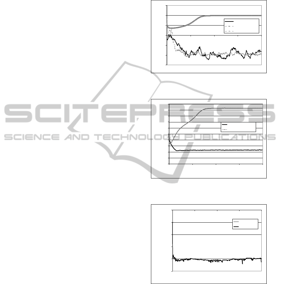
From Figure 5, Figure 6 and Figure 7 it has been
observed that, for all the states and the parameter,
RMS errors of the adaptive GHF converged quickly
to a lower value compared to the non adaptive GHF.
Table 1: Numerical values and description of the
parameters used in simulation.
Symbols Value Description
0
x
[300000 20000 10
-3
]
T
Initial value for
true trajectories
1
q
5 ft
2
s
−3
A parameter of
true Q
2
q
10
-12
ft
−2
s
−1
A parameter of
true Q
M
100000 ft
Horizontal
distance of
object from
radar
H
100000 ft
Height of the
radar
true
R
100
2
ft
2
Measurement
noise
covariance
0
P
diag (10
6
, 4×10
6
, 10
-4
)
Initial a
posteriori error
covariance
0
ˆ
x
N(
0
x ,
0
P
)
Initialization of
filter estimates.
L
100
Actual window
length
This indicates that the AGHF can adapt the
unknown measurement noise covariance and
produces more reliable estimation than non adaptive
GHF in case of the joint estimation of parameters
and states.
1
10
100
1000
10000
0 102030405060
time (sec)
RMS error (ft)
AGHF
Non Adaptive GHF
Figure 5: Comparison of RMS error (altitude estimation)
of AGHF & GHF for 1000 MC runs.
1
10
100
1000
10000
0 102030405060
time (sec)
RMS error (ft/sec)
AGHF
Non Adaptive GHF
Figure 6: Comparison of RMS error (velocity estimation)
of AGHF & GHF for 1000 MC runs.
0.000001
0.00001
0.0001
0.001
0.01
0.1
1
0 102030405060
time (sec)
RMS error (1/ft)
AGHF
Non Adaptive GHF
Figure 7: Comparison of percentage of RMS error
(ballistic parameter estimation) of AGHF & GHF for 1000
MC runs.
5 CONCLUDING DISCUSSIONS
An adaptive Gauss Hermite filter has been proposed
and evaluated with different bench mark nonlinear
estimation problems. It can be inferred from the
results of the Monte Carlo simulation that the
adaptive GHF can successfully adapt the unknown
measurement noise covariance and presents
substantially improved estimation performance over
the non adaptive filter for a wide range of initial
choice of measurement noise covariance. The
suitability of the proposed filter for joint estimation
of parameters and states of nonlinear systems is also
ICINCO2014-11thInternationalConferenceonInformaticsinControl,AutomationandRobotics
588

demonstrated using a well known object tracking
problem.
As the non adaptive GHF reportedly excels other
non adaptive sigma point filters like UKF and CDF,
the performance of the proposed adaptive GHF has
been compared with its non adaptive version.
In the absence of analytical proof of
convergence, each adaptive nonlinear filter,
including the proposed one, are to be thoroughly
evaluated with the help of extensive simulation
studies or real time experiments in several fields of
application before such filtering techniques may be
widely applied in practice with confidence.
However, the proposed filter may be
recommended for state and parameter estimation of
nonlinear systems because of its improved
estimation performance, good convergence, simple
adaptation rule, capacity to accommodate wide
uncertainty in the initial choice of measurement
noise covariance.
ACKNOWLEDGEMENTS
The first two authors acknowledge Council of
Scientific and Industrial Research, New Delhi, India
for financial support and express their gratitude to
the Centre for Knowledge Based System, Jadavpur
University, Kolkata, India for infrastructural
support.
REFERENCES
Simon, D., 2006. Optimal State Estimation: Kalman, H
Infinity, and Nonlinear Approaches, John Wilely &
Sons. New Jersey, 1
st
edition.
Lefebvre, T, Bruyninckx, H., Schutter, J., 2004. Kalman
filters for non-linear systems: a comparison of
performance. In International journal of Control,
77(7), 639-653.
Ito, K., & Xiong, K., 2000. Gaussian filters for nonlinear
filtering problems. In IEEE Transactions on Automatic
Control, 45(5), 910-927.
Arasaratnam, I., Haykin, S., Elliott, R. J., 2007. Discrete-
time nonlinear filtering algorithms using Gauss–
Hermite quadrature. In Proceedings of the IEEE,
95(5), 953-977.
Mehra, R. K., 1972. Approaches to adaptive filtering. In
IEEE Transactions on Automatic Control, 17(5), 693-
698.
Maybeck, P. S., 1982. Stochastic models, estimation, and
control (Vol. 2). Academic Press. New York, 1
st
edition.
Myers, K., Tapley, B. D., 1976. Adaptive sequential
estimation with unknown noise statistics. In IEEE
Transactions on Automatic Control, 21(4), 520-523.
Busse, F. D., How, J., Simpson, J., 2003. Demonstration
of adaptive extended Kalman filter for low earth orbit
formation estimation using CDGPS. In Journal of the
Insitute of. Navigation, 50(2), 79-93.
Das, M., Sadhu, S., Ghoshal, T. K., 2013. An Adaptive
Sigma Point Filter for Nonlinear Filtering Problems.
In International Journal of Electrical, Electronics and
Computer Engineering, 2(2), 13-19.
Karlgaard, C. D., Schaub, H., 2011. Adaptive nonlinear
Huber-based navigation for rendezvous in elliptical
orbit. In Journal of Guidance, Control, and Dynamics,
34(2), 388-402.
Hajiyev, C., Soken, H. E., 2014. Robust adaptive
unscented Kalman filter for attitude estimation of pico
satellites. In International Journal of Adaptive Control
and Signal Processing, 28(2), 107-120.
Dey, A., Sadhu. S., Ghoshal, T. K., 2014. Adaptive Gauss
Hermite Filter for Parameter Varying Nonlinear
Systems. Accepted for presentation in International
Conference on Signal Processing and Communication.
Sadhu, S., Srinivasan, M., Bhaumik, S., Ghoshal, T. K.
2007. Central difference formulation of risk-sensitive
filter. IEEE Signal Processing Letters,14(6), 421-424.
Norgaard, M., Poulsen, N. K., Ravn, O., 2000. New
developments in state estimation for nonlinear
systems. In Automatica, 36(11), 1627-1638.
Athans, M., Wishner, R. P., Bertolini, A., 1968.
Suboptimal state estimation for continuous-time
nonlinear systems from discrete noisy measurements.
In IEEE Transactions on Automatic Control, 13(5),
504-514.
Ristic, B., Farina, A., Benvenuti, D., Arulampalam, M. S.,
2003. Performance bounds and comparison of
nonlinear filters for tracking a ballistic object on re-
entry. In IEE Proceedings Radar, Sonar and
Navigation, 150(2), 65-70.
AdaptiveGaussHermiteFilterforParameterandStateEstimationofNonlinearSystems
589
