
Reconfigurable Wireless Sensor Networks
New Adaptive Dynamic Solutions for Flexible Architectures
Hanen Grichi
1
, Olfa Mosbahi
2
and Mohamed Khalgui
2
1
Tunisia Polytechnic School, La Marsa, Tunisia
2
National Institute of Applied Science and Technology, University of Carthage, Tunis, Tunisia
Keywords:
Wireless Sensor Network, Reconfiguration, Multi-agent Architecture, Nested State Machine, Simulation.
Abstract:
This paper deals with reconfigurable wireless sensor networks RWSN that should be adapted to their envi-
ronment under user and energy constraints. A RWSN is assumed to be composed of a set of communicating
nodes such that each one executes reconfigurable software tasks to control local sensors. We propose three
reconfiguration forms to adapt a RWSN: (a) software reconfiguration allowing the addition/ removal/ update of
tasks, (b) hardware reconfiguration allowing the activation/deactivation of nodes, (c) protocol reconfiguration
allowing the modification of routing protocols between nodes. We propose a zone-based multi-agent architec-
ture for RWSN where a communication protocol is well-defined to optimize distributed reconfigurations. Each
agent of this architecture is modeled by nested state machines in order to control the problem complexity. The
paper’s contribution is applied to a case study that we simulate to show the originality of this new architecture.
1 INTRODUCTION
Wireless Sensor Networks (to be denoted by WSN)
become today an important established technology
for a large number of applications (pollution pre-
vention (Vikram Guptay and Tovary, 2011), agricul-
ture (Wang, 2010), military, structures and buildings
health, etc). WSNs usually consist of many small de-
vices called sensor nodes. Each node is able to allow
local control processing and communications with re-
mote nodes under real-time and energy constraints.
Wireless Sensor Networks can be homogeneous (sen-
sor nodes are of the same nature) or heterogeneous
(with different types of nodes) (R.Saravanakumar,
2011). We are interested in this paper in homo-
geneous WSN. Several related works such as (Hnin
Yu Shwe and Kumar, 2013), (Mahalik, 2009) de-
scribe the wireless sensor network (WSN) as a sys-
tem of spatially distributed sensor nodes that col-
lect important information in the target environment.
Each sensor node has limited computation capacity,
local memory, power supply (Swamy, 2003) and com-
munication link. Each directed link connects two
neighboring nodes through a network (T.-S. Chen
and Sheu, 2000). The most generic model for a
WSN is based on the data gathering (Jiping Xiong
and Chen, 2013) and communication capabilities
of sensors. Nowadays, WSN migrate to an auto-
programming technology which is based on intelli-
gent sensor networking infrastructures (Vikram Gup-
tay and Tovary, 2011). The system can change its
behavior at run-time, it is what we call a reconfig-
urable system. Two reconfiguration policies could
be identified: static (offline: by stopping the WSN
to make required modifications and restart it) or dy-
namic (online: by changing the network structures
during its execution) (R.Saravanakumar, 2011). In the
second case, we have also two kinds of reconfigura-
tion: manual (executed by users) and automatic (ex-
ecuted by agents). The researchers define the RWSN
(Reconfigurable WSN) as an adaptive WSN. The re-
configuration is any operation that redirects data flows
when we change the state of source or destination
nodes. The reconfiguration can also add/remove
one/more physical elements of the network by activat-
ing/deactivating them. The reconfiguration touches
first the material (allowing the activation/deactivation
of nodes), second the software (allowing the recon-
figuration of tasks) and third the communication pro-
tocols (allowing the adaptation of routing protocols
between nodes). Many projects deal with RWSN
such as WASAN (Kindratenko1 and Pointer, 2005),
ReWINS (Harish Ramamurthy, 2005), TWIST project
(Vlado Handziski, 2005). This definition touches one
or two reconfiguration types (hardware, software or
protocol) but these works do not mix all of them. Our
254
Grichi H., Mosbahi O. and Khalgui M..
Reconfigurable Wireless Sensor Networks - New Adaptive Dynamic Solutions for Flexible Architectures.
DOI: 10.5220/0005005602540265
In Proceedings of the 9th International Conference on Software Engineering and Applications (ICSOFT-EA-2014), pages 254-265
ISBN: 978-989-758-036-9
Copyright
c
2014 SCITEPRESS (Science and Technology Publications, Lda.)

problem consists in the application of these three re-
configuration types: what is the gain that we can get
by using any hardware reconfiguration, or software
reconfiguration or also the protocol reconfiguration?
If we reduce the communication by applying recon-
figuration scenarios, can we win in term of energy?
We try in this paper to answer these questions by
defining three forms of reconfiguration for low power
RWSNs. We define a new zone-based multi-agent ar-
chitecture for RWSN where a communication proto-
col is well-defined for useful distributed reconfigu-
rations. We decompose the RWSN to a set of zones
where each one gathers a number of nodes. The radius
of each zone is a parameter to be defined by users ac-
cording to several characteristics of the followed tech-
nology. We define a Controller Agent (CrA) that han-
dles the reconfiguration strategies of the whole net-
work, and assign a Zone Agent for each zone (ZA) to
control the local reconfiguration scenarios. Each node
of a particular zone is controlled by a Slave Agent
(SA) that monitors the local reconfiguration scenarios
inside the node. This original multi-agent architec-
ture combines all possible reconfiguration forms to
be adapted for the environment where we minimize
the energy consumption. This adaptive architecture
is modeled by nested state machines in order to con-
trol the specification complexity. With our solution,
we gain in term of energy to be consumed by each
node and the number of exchanged messages between
nodes in the network. This architecture supports the
delegation between agents and controls the complex-
ity by providing hierarchical structure of RWSN. We
apply and simulate the paper’s contribution to a case
study to be assumed as a running example, and com-
pare our results to some related works in order to
show the originality of this architecture.
The paper is organized as follows: after introduc-
tion and background, Section 3 presents our position
between related works. Section 4 proposes a new def-
inition of RWSN to be explained on a case study. The
multi-agent architecture of the RWSN is proposed in
Section 5. Section 6 presents the coordination pro-
tocol between different agents. The simulation and
evaluation of the paper’s contribution is provided in
Section 7 before concluding the paper in Section 8.
2 BACKGROUND
We briefly present the formalism of finite state ma-
chines to be used in the following for the modelling
of RWSN. Finite State Machine (FSM) is an abstract
machine that can be in one of finite number of states.
It changes the behavior from a state to another by fir-
ing a transition in response to particular event. A FSM
is an efficient way to specify constraints of the over-
all behavior of a system (Samek, 2003). A classic
form of a FSM is a direct graph with the following el-
ements: G=(Q, Σ, Z, δ, q
0
, F) where: (a) Vertices Q is
a finite set of states (Q
1
,Q
2
,...,Q
i
) such that each state
(Q
i
) models a system’s behavior at an instant t, (b) In-
put symbols Σ is a finite collection of input symbols
or designators. This part of graph represents the finite
set of initial states, (c) Output symbols Z is a finite
collection of output symbols or designators. This part
of graph represents the final state of the system, (d)
Edges δ represents transitions from one state to an-
other as caused by input symbols, (e) Start state q
0
is
the start state q
0
∈ Q, (f) Accepting state(s) F: F ∈ Q
is the set of accepting states. We define Nested State
Machines as a set of FSM such that a state of one cor-
responds to another machine. This solution is useful
for the modeling of a complex system where the in-
formation should be modeled on different hierarchical
levels in order to control the complexity.
3 STATE OF THE ART
Today, several researches deal with RWSN where a
reconfiguration can be applied in three levels: hard-
ware, software and data routing (Bellis et al., 2005),
(Jie CHEN and LUO, 2009). Hardware recon-
figurations are defined in (Bellis et al., 2005) by
adding FPGA-based intelligent modules to nodes. In
(Kindratenko1 and Pointer, 2005), the wireless au-
tonomous sensor and networks of actors (WASAN)
define hardware reconfigurations as dynamic oper-
ations that model platforms of evaluation and assis-
tance. To model well the protocol reconfiguration,
the existence of reconfigurable interfaces is essential;
Harish Ramamurthy in (Harish Ramamurthy, 2005)
presents the ReWINS project (Reconfigurable Wire-
less Interface for Networking), to manage the recon-
figurability thanks to a ’Central Control Unit’. The
Reconfigurable Wireless Sensor Network for Struc-
tural Health Monitoring (M. Bocca and Eriksson,
2009), is also another project of RWSN. This proposi-
tion has the possibility to reconfigure the parameters
of the monitoring application (software reconfigura-
tion), depending on the needs of the end-user oper-
ating at the sink node. To optimize the radio trans-
mission of data and avoid interferences (protocol re-
configuration), each sink node establishes a reserved
communication link with each of the sensor nodes. In
(Vlado Handziski, 2005), the TWIST project (a scal-
able and flexible tested architecture for indoor deploy-
ment of wireless sensor networks) defines two recon-
ReconfigurableWirelessSensorNetworks-NewAdaptiveDynamicSolutionsforFlexibleArchitectures
255

figuration forms: software/ hardware. This project
uses the USB infrastructure for the hardware recon-
figuration and the software one is controlled by a set
of interfaces to be implemented on a station.
We note that all related works do not address all
possible reconfiguration forms together that the cur-
rent paper deals with: software, hardware and pro-
tocol reconfigurations. We propose a new zone-
based multi-agent architecture for RWSN. Our propo-
sition is original and different from all others since we
treat all reconfiguration forms, control the complex-
ity of modeling by using nested state machines and
optimize the energy consumption as well as the ex-
changed messages between nodes thanks to the zone-
based solution.
4 CONTRIBUTION: NEW
SOLUTIONS FOR RWSN
4.1 RWSN: Definition
We define a reconfiguration scenario as any response
to a request in order to adapt the system to its en-
vironment and to improve also its performance. We
consider three kinds of reconfigurations: (i) soft-
ware reconfiguration allowing the addition/removal
and update of Os-tasks or data, (ii) hardware recon-
figuration allowing the activation/deactivation of sen-
sor nodes, (iii) protocol reconfiguration allowing the
optimization/degradation of the protocol (e.g. addi-
tion/removal/update of messages to be exchanged be-
tween nodes as well as their routing paths). We denote
in the following by a RWSN, a reconfigurable WSN
that automatically modifies its software and/or hard-
ware architecture and/or inter-nodes communication
protocol. Contrary to all related works, a RWSN is
defined as a dynamic reconfigurable WSN, that auto-
matically modifies at run time the architecture as well
as structure of the network. This modification can
touch the material (e.g. sensors), the software (e.g.
OS tasks) and the data routing. Note that the TWIST
project (Vlado Handziski, 2005) does not address the
protocol reconfiguration. The ReWINS project (Har-
ish Ramamurthy, 2005) does not suppose the recon-
figuration of WSN as a dynamic and automatic recon-
figuration. In the current paper, we extend all related
works and address all possible reconfiguration forms
that can be applied at run time on RWSN.
4.2 RWSN: New Architecture
We give in the following some definitions that will be
used in the following.
• RWSN: a set of Nbz zones and S stations. A station
controls the whole network, whereas each zone is
composed of n nodes such that each node gath-
ers m hardware detectors to be controlled by soft-
ware tasks. Note that a communication protocol
is applied between nodes of a same or of different
zones. We define Nbz = number of the zones in
WSN and Zi as the zone number i of the network.
• RWSN zone: a geographical space to be defined
by all the points included in the area of this zone.
This zone is fixed by a radius to be defined by the
RWSN designer.
• RWSN station: a supervisor in a RWSN to be char-
acterized by: (i) A memory, that should be bigger
than a node memory, (ii) A bandwidth, that repre-
sents the velocity of data transmission with nodes.
• Reconfigurable node: a device to be composed
with others. It runs under energy, real-time and
functional constraints. A node is characterized by:
(i) An identifier (ID) which is unique in the zone,
(ii) a set of m detectors DTi (i =1,2,...,m) where
each sensor is modeled by two variables: the state
(Sd: active or not), and the value to be detected
(Vd), (iii) a power unit represented by two batter-
ies (we denote by PwBi(t) the current value of bat-
tery’s charge and PwBiMax the maximum load),
(iv) the router (R) that supports the communica-
tions with other nodes.
• Reconfigurable sensor: a detector that consumes
energy to provide required services for the node.
We suppose that it is controlled by a unique OS-
Task.
• Reconfigurable protocol: a protocol that supports
the communication between nodes. We assume it
as reconfigurable since we suppose that messages
can be added or removed at run-time. Table 1 de-
scribes the parameters of a routing table in each
node in order to characterize each communication
between them.
Table 1: Node routing table parameters.
ID Node Identifier
IDZone Zone Identifier
IDDest Final Destination Node Identifier
IDNext Next Node Identifier in communication
path (neighbor)
Time Execution time for communication by
a node
4.3 Reconfiguration Forms
We have three forms of reconfigurations:
ICSOFT-EA2014-9thInternationalConferenceonSoftwareEngineeringandApplications
256
4.3.1 Software Reconfiguration
Modifies the behaviors of nodes at run time. The
modification is made on the software architecture by:
(i) adding (or removing) OS-tasks to be executed in
nodes, (ii) modifying their scheduling, (iii) modify-
ing the used data by tasks.
4.3.2 Hardware Reconfiguration
This kind of hardware reconfiguration consists of:
(i) activation/deactivation of detectors, (ii) activa-
tion/deactivation of nodes. The deactivation of all
detectors in a node implies its deactivation. In fact,
activating only one detector in a node results in its ac-
tivation.
4.3.3 Protocol Reconfiguration
Consists in modifying the data routing when soft-
ware and hardware reconfigurations are applied at
run-time.
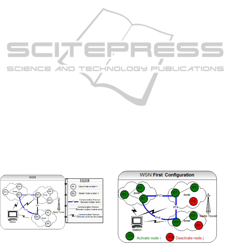
4.4 Case Study
We propose as a running example a RWSN to be de-
noted by Sys. It is composed of 3 zones (Z1, Z2,
Z3) where each one Z
i
is composed of three nodes.
These three zones are supervised by a station (S).
Each node Nzj, ( j = 1..9) is characterized by two de-
tectors, two batteries and a router (Rj). Each detec-
tor DTm, (m = 1 or 2) can detect the temperature (to
be denoted by DT1) and the humidity of the environ-
ment (to be denoted by DT2). It is characterized by
a state (Sd: {activate= 1, deactivate= 0}), and the de-
tected value (Vd). The two batteries are denoted by
Bk(k = 1 or 2). Each battery Bk is characterized by
a current value of load (PwBk,j) and a value of maxi-
mum load (PwBMaxk,j). We suppose initially, that Nz5
executes only DT1(see Figure 1).
Figure 1: A Case Study of an WSN.
4.4.1 Software Reconfiguration
We define the following three tasks {T1,T2,T3}: (i)
T1: controls the temperature and detects signal when
it is higher than 45
◦
C. (ii) T2: reduces the threshold
from 45
◦
C to 30
◦
C. This task can be used for any
detection of fire. (iii) T3: controls the humidity of the
environment. We define 3 software reconfigurations:
{SR1, SR2, SR3}. (a) SR1: a reconfiguration that al-
lows the addition of (T1) to each node in a summer
day; (b) SR2: is applied to each summer night to re-
move the task (T1) and to add (T2). (c) SR3: updates
the threshold to be taken by (T3).
4.4.2 Hardware Reconfiguration
In order to minimize the dissipated energy, we ap-
ply hardware reconfigurations {HR1, HR2, HR3} on
3 sensor nodes (Nz1 from Z1, Nz5 from Z2, Nz9 from
Z3) (i) HR1: deactivates Nz1 from Z1 by deactivating
(DT1(1) of Nz1 and DT2(1) of Nz1), (ii) HR2: deacti-
vates DT1(5) for the node Nz5, (iii) HR3: activates Nz9
from Z3 by activating DT2(9) of Nz9. The hardware
reconfiguration, in this case, can change the routing
information between nodes. The link of communica-
tion between Nz1 and its neighbors is cut (the same
case as Nz5). By using HR3, (Nz9) can be connected
to its neighbors (see the modification from Figure 2 to
Figure 3).
4.4.3 Protocol Reconfiguration
If we apply HR1, HR2 and HR3 (deactivation of Nz1,
Nz5 and activation of Nz9), the routing tables of (Nz1,
Nz5, Nz9) will be changed from Table 2 to Table 3. In
this case the reconfiguration of protocol eliminates 3
communication links between nodes (Nz1, Nz5), and
adds 2 other links to (Nz9).
Figure 2: First configuration of (WSN).
ReconfigurableWirelessSensorNetworks-NewAdaptiveDynamicSolutionsforFlexibleArchitectures
257
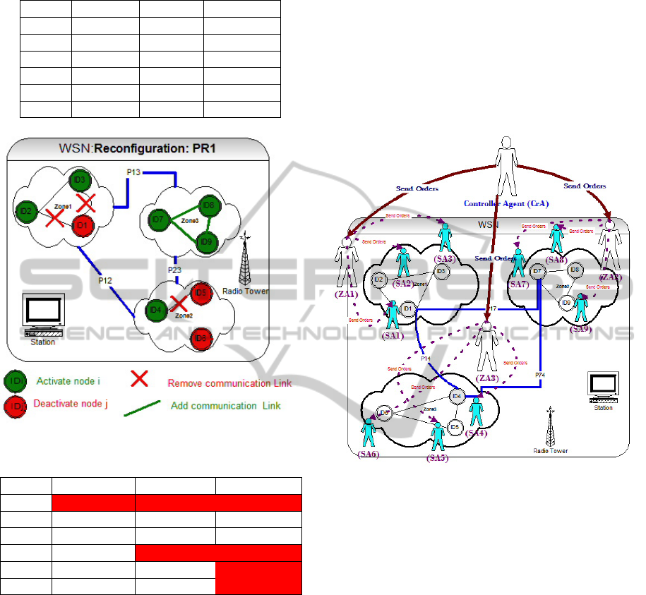
Table 2: First routing table parameters.
Nz1 Nz5 Nz9
State Activate Activate Deactivate
ID ID1 ID5 ID9
IDZone Z1 Z2 Z3
IDDest ID7 ID1
IDNext ID2, ID3 ID4
Time 0.02s 0.01s
Figure 3: Protocol reconfiguration of (WSN).
Table 3: Second routing table parameters.
Nz1 Nz5 Nz9
State Deactivate Deactivate Activate
ID ID1 ID5 ID9
IDZone Z1 Z2 Z3
IDDest ID7 ID9 ID2
IDNext ID2 Or ID3 ID4 ID7 Or ID8
Time 0.02s
5 NEW MULTI-AGENT
ARCHITECTURE FOR (RWSN)
5.1 Motivation
To handle all cited forms, we propose a multi-agent
architecture for RWSN. This architecture is composed
of a Controller Agent (CrA) that controls the whole
architecture, a Zone Agent (ZA) to be affected to each
zone in order to control its nodes, and a Slave Agent
(SA) that controls each node of any zone. All these
agents handle the different reconfiguration forms that
we described above. In order to control the com-
plexity, each agent has a hierarchical architecture to
be modeled by Nested State Machines. We show in
Figure 4 this new multi-agent architecture of RWSN.
We model the multi-agent architecture for RWSN as a
system to be composed by one CrA, a set of (ZA) and
a set of (SA): Sys={CrA, ϕZA, ϕSA};
ϕZA= set of all Zones Agents;
ϕSA = set of all Slaves Agents;
In one Zone = {ZA, ϕSA}
Figure 4: Multi-Agent Architecture for RWSN.
We denote in the following by SetZi the set of all mas-
ter and slave nodes in the zone i. Let we assume a
node Nzji of the zone i, it is denoted by Snji if it is the
jth slave node of this zone and by Mnji if it is the j
master one.
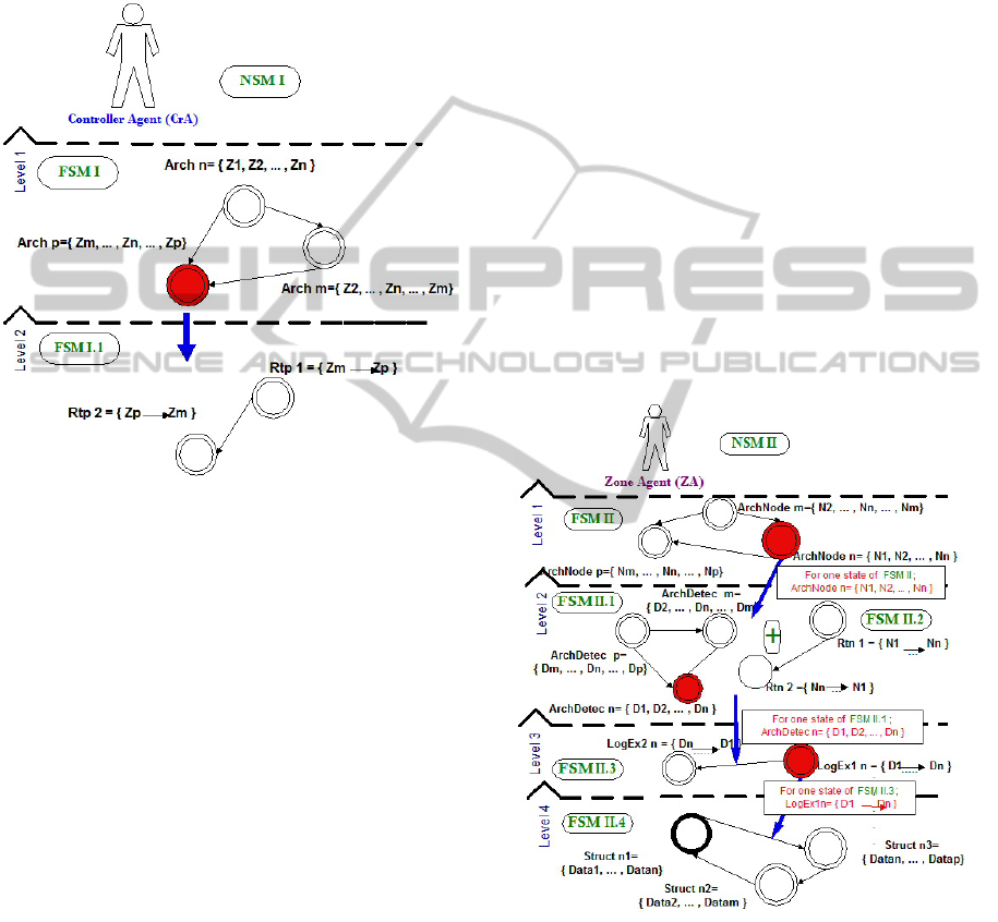
5.2 Formalization of RWSN
5.2.1 Controller Agent (CrA) Logic
For the modeling of this agent, we propose two lev-
els: (i) First Reconfiguration Level: CrA Architec-
ture: The (CrA) defines in this level the set of active
and deactive zones under well-defined conditions at
a particular time. This level will be modeled latter
with the State Machine (FSM I). (ii) Second Recon-
figuration Level: CrA Data Flows: This level de-
scribes the different flows of data to be exchanged
between the active zones that we define in level 1.
For each state of (FSM I) that models level 1, we de-
fine in the current second level a particular state ma-
chine that defines all the possible data flows. A state
ICSOFT-EA2014-9thInternationalConferenceonSoftwareEngineeringandApplications
258
of this State Machine defines a particular reconfigura-
tion scenario that changes the routing policy software
between zones. In Figure 5, the red state of (FSM
I) defines a subset of active zones and corresponds to
the state machine (FSM I.1) in level 2. The state Rtp 1
represents a first routing solution between these zones
and Rtp 2 represents another routing solution.
Figure 5: Controller Agent architecture.
5.2.2 Zone Agent (ZA) Logic
We propose four levels for this agent: (i) first recon-
figuration level: ZA Architecture: we describe in
this level the different active and deactive nodes under
well-defined conditions at a particular time. This level
is characterized by a superset of nodes such that any
reconfiguration scenario corresponds to the activation
of a subset, (ii) second reconfiguration level: ZA
Data Flows/ Detectors: the second level of the Zone
Agent (ZA) defines the set of detectors that should be
active in each node under well-defined conditions at
a particular time. This second level defines also the
different data flows that can be followed to exchange
data between the active nodes of the zone. The activa-
tion of detectors as well as the definition of reconfig-
uration data flows belong to the same level since they
are depending in logic, (iii) third reconfiguration
level: ZA Scheduling: this level defines the different
reconfigurable scheduling of OS-tasks that control ac-
tive detectors in active nodes under well-defined con-
dition at a particular time, (iv) fourth reconfigura-
tion level: ZA Data value: This level defines the dif-
ferent values and structure of data to be used by the
OS-tasks of active nodes under well-defined condi-
tions at a particular time.
To handle the complexity of the problem, we use
nested state machines to model the Zone Agent. In
Figure 6, the red state ArchNode n defines the differ-
ent active nodes of a zone at a particular time t un-
der well-defined conditions, this state corresponds to
two state machines FSM II.1 and FSM II.2 in level 2.
FSM II.1 defines in this zone all possible activations
of detectors. FSM II.2 represents the different routing
solutions between active nodes in this zone. The red
state ArchDetect n defines under well-defined condi-
tions the different detectors which should be active in
active nodes of the zone. Rtn 1 defines a particular
solution to exchange data between active nodes in a
zone. Two states of these state machines of level 2
define a particular state machine in level 3 where a
state defines a particular scheduling of active tasks.
The red state LogEx1 n defines the execution logic
of tasks and defines a new state machine FSM II.4 in
level 4. Each state in FSM II.4 defines particular val-
ues and structures of data to be used by actives tasks.
Thanks to this solution we can cover all possible re-
configuration forms while controlling the complexity
of the problem.
Figure 6: Zone Agent architecture.
5.2.3 Slave Agent (SA) Logic
This agent executes the reconfiguration strategies to
be defined by CrA and ZA.
Note Finally that to gain in terms of energy for ex-
ample, each Zone Agent (ZA) controls at run-time the
load in the batteries of each slave before applying re-
quired reconfiguration scenarios that can possibly re-
ReconfigurableWirelessSensorNetworks-NewAdaptiveDynamicSolutionsforFlexibleArchitectures
259

move tasks or also deactivate nodes in order to pre-
serve power as much as possible. We note also that we
are interested in the architecture of RWSN without de-
tailing the technical solutions to add/remove tasks or
activate/deactivate nodes. We are not interested also
in the real-time scheduling of tasks that will be in an-
other paper. The contribution of the current paper is
dealing with the architecture of RWSN to address all
possible reconfiguration forms while controlling the
complexity of the problem.
5.3 Modeling of RWSN
5.3.1 Controller Agent (CrA) Model
We model the two levels of (CrA) by the following
state machines.
-First modeling level: CrA Architecture:
GC
1
=(Qc, δc, qc
0
) where:
(a) Vertices Qc: set of states such that each
state corresponds to active zones at a partic-
ular time (Qc
1
,Qc
2
,...,Qc
i
). We denote by
Qc
i
=(MN
1
,MN
2
,...,MN
n
) the set of active master
nodes of RWSN, (b) Edges δc: activation or deacti-
vation of master nodes, (c) Start state qc
0
: a first
architecture which defines the default active zones.
-Second modeling level: CrA Data flows: For each
state Qc
i
∈ Qc in GC1, we define:
GC
2
=(Qp, δp, qp
0
) where:
(a) Vertices Qp: set of states where each one rep-
resents a particular routing solution between active
zones (Qp
i1
,Qp
i2
,...,Qp
i j
). (b) Edges δp: the mod-
ification of data flows between active zones. (c) Start
state qp
0
: the data flows between the default active
zones.
Figure 7 describes (FSM I) and (FSM I.1) that
model level 1 and level 2 for CrA:
5.3.2 Zone Agent (ZA) Model
We define the following nested state machines of each
(ZA).
First modeling level: ZA Architecture:
GD
1
=(Qd, δd, qd
0
) where:
(a)Vertices Qd: set of states such that each
one represents a subset of active nodes in a
zone, Qd
i
=(N
1
,N
2
,...,N
i
), (c)Edges δd: activa-
tion/deactivation of nodes in a zone, (d)Start state
qd
0
: default list of nodes in a zone.
Second modeling level: ZA Data flows/detectors: For
each state Qd
i
of GD
1
, we define two state machines
GN
2
and GN
0
2
:
Figure 7: CrA Running Example.
GN
2
=(Qn, δn, qn
0
) where:
(a)Vertices Qn: set of states where each one rep-
resents a particular routing solution between active
nodes of a zone, (b)Edges δn: modification of data
flows between active nodes, (c)Start state qn
0
: data
flows between default active nodes Qn
i1
.
GN
0
2
=(Qn’, δn’, qn
0
0
,) where:
(a)Vertices Qn’: set of states such that each
one represents detectors to be active at a par-
ticular time ,(Qn
0
i1
,Qn
0
i2
,...,Qn
0
i j
). We can define
Qn
0
i j
=(Detc
1
,Detc
2
,...,Detc
n
) as a set of active detec-
tors, (b)Edges δn’: activation/deactivation of detec-
tors, (c)Start state qn
0
0
: the default list of detectors in
a node: Qn
0
i1
.
Third modeling level: ZA Scheduling: For each state
Qn
i j
in GN
2
and Qn
0
i j
in GN
0
2
, we define:
GE
3
=(Qe, δe, qe
0
) where:
(a)Vertices Qe: set of states such that each one rep-
resents the scheduling of OS-tasks implementing ac-
tive nodes in a zone. ,(Q
i j1
,Q
i j2
,...,Q
i jk
), (b)Edges
δe: modification of the execution sense of detectors
by respecting the dependence of the latter, (c)Start
state qe
0
: the default scheduling of OS-tasks Qe
i j1
Fourth modeling level: ZA Data value: For each state
Qe
i jk
in GE
3
, we define:
GS
4
=(Qs, δs, qs
0
) where:
(a)Vertices Qs: set of states where each state repre-
sents data structures and values to be used by active
tasks, (Q
i jk1
,Q
i jk2
,...,Q
i jkl
), (b)Edges δs: modifica-
tion of data structure or values, (c)Start state qs
0
: the
default data structures Q
i jk1
.
Figure 8 defines the nested state machines that
model ZA1 of Z1. FSM II is a state machine that
ICSOFT-EA2014-9thInternationalConferenceonSoftwareEngineeringandApplications
260
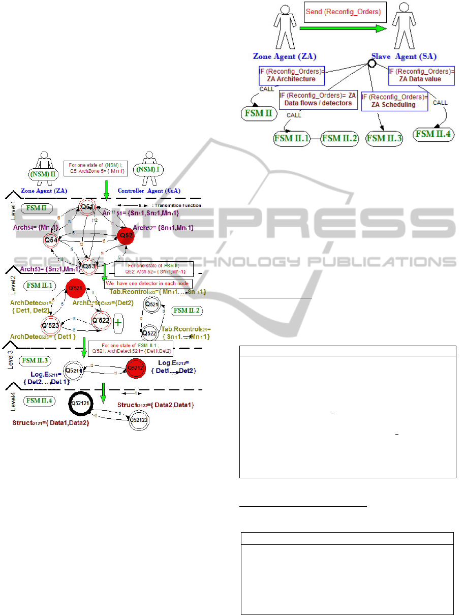
defines all possible activations of nodes in the zone,
the red state Q52 corresponds to two state machines
FSM II.1 and FSM II.2 in level 2. Q
521
represents a
particular data flow between active nodes in a zone.
Q
521
is a set of active detectors in a node. Both of the
two states correspond to a particular state machine in
level 3 . Q
5212
represents a particular scheduling of
OS-tasks that control active detectors in level 2. Q
5212
corresponds to particular data structures FSM II.4 in
level 4, Q
52121
corresponds to a particular data struc-
tures and values to be used by active nodes in this
zone Zone1.
Figure 8: Running Example for ZA Modeling.
5.3.3 Slave Agent Modeling (SA)
This agent executes directly the orders of the corre-
sponding (ZA). Figure 9 shows the reaction of a slave
agent in Zone1 when it receives an order from a cor-
responding Zone Agent.
6 COORDINATION PROTOCOL
BETWEEN AGENTS
We propose a communication protocol between the
different agents (CrA, ZA, SA) of this architecture. It
is based on the following operation: (i) CrA Algo-
rithm: the operation that links CrA to any ZA. (ii) ZA
Figure 9: Running Example for SA Modeling.
Algorithm: the operation between any ZA and any cor-
responding SA. (iii) Oper 1: an operation allowing the
activation/deactivation of nodes in a zone. (iv) Oper2:
an operation allowing a modification of data flows in
a zone (v) Oper3: an operation allowing the activa-
tion/deactivation of detectors in a node. (vi) Oper4:
an operation allowing the modification of scheduling
in a zone and (vii) Oper5: an operation allowing the
modification of data structures or values in a zone.
CrA Algorithm: to apply a reconfiguration, CrA
sends to any ZA an array containing the list of de-
sired active zones with the new flow of data to be ex-
changed between them.
Algorithme 1 : CrA Algorithm
Z Zone; newArray(tabZoneActiv[nb]);
DS= Transmission Distance (threshold);
D(CrA,j)= α, j 6= CrA;
D(i,j)=β , j 6= i;
REPEAT
{Send new vector(activ zones) to neighbors zones:
IFD(CrA,j) ≤ DS; Send (tabZoneActiv[nb], CrA, j);
FOR EACHdest j, find the next with dist min to j;
IFD(i,j) ≤ DS; Send(tabZoneActiv[nb], j, i);
i+1; calculate(D(i,j));}
UNTIL D (i,j)= 0; source i = destination j;
Send(ProtoCommunic (AC, ZoneDest1, ..., ZoneDestj));
ZA Algorithm: Step-By-Step (ZA) sends to any
(SA) a reconfiguration scenario.
Algorithme 2 : ZA Algorithm
We declare: VAR = orderReconfig(ZA, SA);
IF (VAR =1) Send (ReconficArchitecNode(), ZA, SA);
IF (VAR =2) Send (ReconfProtoCommNod(), ZA, SA);
IF (VAR =3) Send (ReconfArchiDetectors(), ZA, SA);
IF (VAR =4) Send (ReconfLogicExecDetec(), ZA, SA);
IF (VAR =5) Send (ReconficStructData(), ZA, SA);
ReconfigurableWirelessSensorNetworks-NewAdaptiveDynamicSolutionsforFlexibleArchitectures
261

7 SIMULATION AND
EVALUATION
In order to show the benefits of the paper’s contribu-
tion, we apply a simulation of RWSN. We start with
a theoretical simulation before presenting a practical
one.
7.1 Theoretical Simulation
We propose a system (Sys) to be composed of 10
zones (Z1...Z10), each one is composed of 100 nodes:
one master node (Mni) and 99 slaves (Snj), and a
station (S) to control the whole RWSN. Each node
Nz(j) in the same zone Zi is characterized by two
sensors or detectors : DT n
j
(n =1 or 2) to detect the
temperature and the humidity of the environment.
Each sensor node is equipped with a battery, thus
the available energy is limited. Our system (Sys) is
characterized as follows: (i) all the nodes (Nzn) are
homogeneous in terms of battery and transmission
range, (ii) an omnidirectional antenna is installed
in each sensor node and the transmission range is
defined in 15m (DS), (iii) each node is identified by
a unique identifier in the network, (iv) the data are
transmitted without any delay, (v) the exchanged
messages are with a constant size. To Apply the three
forms of reconfiguration, we execute the following
scenarios: (i) (CrA) sends the first reconfiguration
to be applied: activation of all nodes (Hardware
reconfiguration) and modification of temperature to
be (45
◦
C) (Software reconfiguration), (ii) (ZA) of
each zone receives this order and broadcasts it to each
corresponding slave which applies this order, (iii)
(SA) verifies the new routing table according to the
recommendation of ZA (Protocol reconfiguration),
(iv) All (SA) send the collected information in step by
step to (CrA). This scenario is described as follows:
ICSOFT-EA2014-9thInternationalConferenceonSoftwareEngineeringandApplications
262
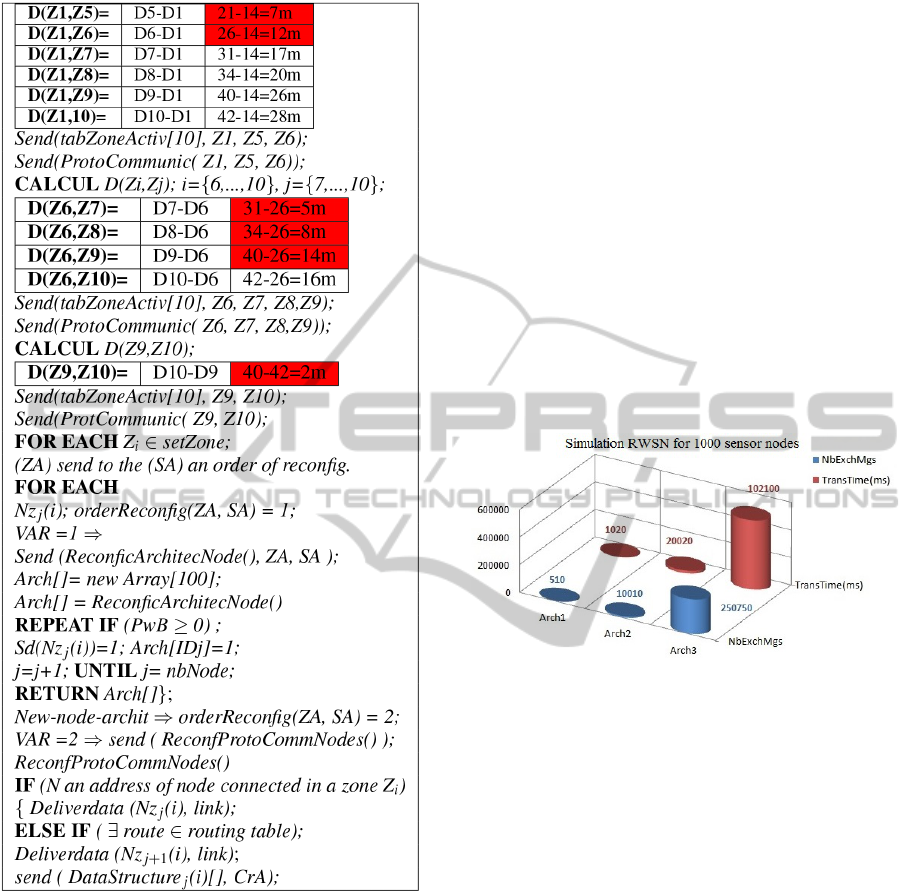
To show the benefits of our contribution,
we compare this work to the projects TWIST
(Vlado Handziski, 2005) and ReWINS (Harish Ra-
mamurthy, 2005): (i) we compute the number of ex-
changed messages in our multi-agent architecture of
RWSN (denoted by Arch 1) where 10 messages are
exchanged between (CrA) and the 10 (ZA) agents. We
suppose that we have 50 active nodes and 50 deac-
tive ones per zone. In this case, 50 messages are
exchanged between (ZA) and (SA). The number of
exchanged messages: NbExchMgs1= 10+10*50=510
messages. For the TWIST project (Vlado Handziski,
2005), the authors use the notion of Super nodes,
(denoted by Arch 2), which is similar to our Zone
Agent but without a concept of active nodes. We
have 10 messages to be exchanged between the sta-
tion and super nodes (10 messages are equal to the
number of super nodes) plus the messages to be ex-
changed between the super nodes and all others=
10*1000. The number of exchanged messages is
NbExchMgs2= 10+10*1000=10010 messages. For
the project ReWINS (Harish Ramamurthy, 2005),
the authors do not consider an agent-based architec-
ture. We denote this architecture by Arch 3, we have,
500 exchanged messages between the station and its
nearly nodes plus the exchanged messages between
the rest of nodes. The number of exchanged messages
is NbExchMgs3= 500+
500
∑
i=0
i=250750 messages. mes-
sages. (ii) If we suppose that the time of transmission
of any message is 2 ms, we can calculate the trans-
mission time of all messages for these three solutions
as follows.
Figure 10: .Comparison between 3 architectures types:Arch
1, Arch 2, Arch 3.
Note that the minimization of exchanged mes-
sages between nodes reduces the total energy con-
sumption in a RWSN. We can compute the com-
plexity of our coordination protocol that we com-
pare to related works (Vlado Handziski, 2005) and
(Harish Ramamurthy, 2005). Let n be the constant
size of data to be exchanged between nodes, and N
be the number of operations in the communication
protocol (Oper 1, Oper 2, Oper 3, Oper 4, Oper 5),
Nb(oppj) the number of sub-operations in the op-
eration oppj, j=(A,..5), Size(n): the algorithm size
or the total number of sub-operations in the proto-
col. The complexity of our protocol is compared
to related works (Vlado Handziski, 2005) and (Har-
ish Ramamurthy, 2005) as follows: (a): For our ar-
chitecture (Arch 1): Size(n) =
5
∑
j=1
(
n
∑
i=0
Nb(opp j)) =
5(2n[log
2
n]) = 10n[log
2
n] and the complexity is
O(10n[log
2
n])=O(n[log
2
n]). The Size(n)=recursive
equation. (b): For TWIST (Vlado Handziski, 2005)
architecture (Arch 2), we have: Size(n)= n(2n[log
2
n])
= n
2
[log
2
n] and the complexity is O(n2[log
2
n]). (c):
ReconfigurableWirelessSensorNetworks-NewAdaptiveDynamicSolutionsforFlexibleArchitectures
263
For ReWINS (Harish Ramamurthy, 2005) architec-
ture (Arch 3), we have: Size(n) = n
3
and the complex-
ity is O(n
3
).
7.2 Practical Simulation
We are interested in the exchange of signals between
nodes when the temperature is between 30
◦
C and
50
◦
C (30
◦
C ≤Temp≤ 50
◦
C). Our major goal is
to keep all nodes of the network on live as much
as possible. We assume that if the number of dead
nodes (node with battery charge = 0, PwB=0) reaches
30% of the original number of nodes (in order of 300
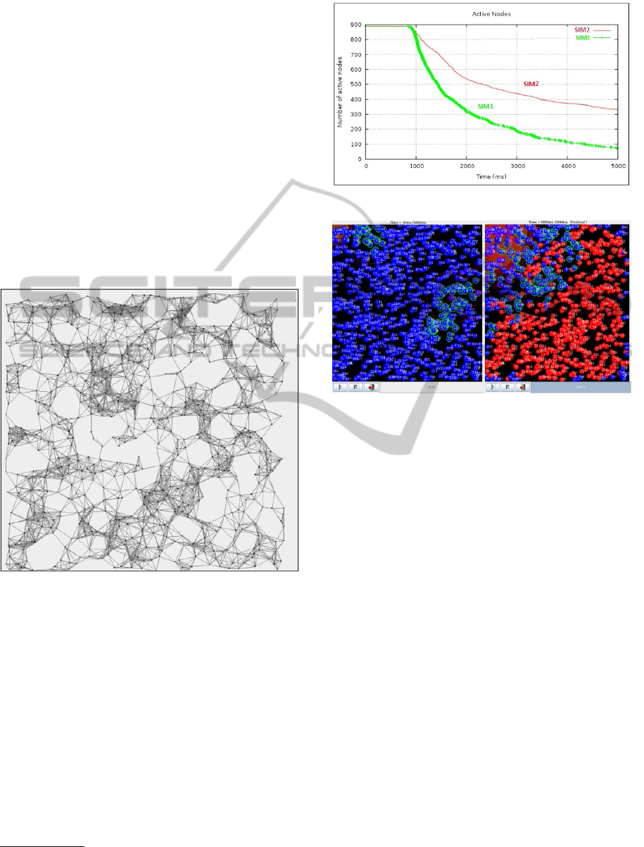
nodes) then, the network collapses. We apply our con-
tribution to this case study by using WSNet (Wire-
less Sensor Network simulator) (Elyes Ben Hamida,
2007). Figure 11 shows the network topology
1
.
Figure 11: Simulated RWSN topology.
We assume two simulation strategies: (i) First
case (SIM1): We suppose that we do not apply the pa-
per’s contribution. Each node sends periodically the
temperature information even it’s higher than 50
◦
C,
(ii) second case (SIM2): We apply our contribution by
assuming that each node stops any emission of tem-
perature information if it is higher than 50.
Figure 12 shows the benefits of our contribution
that we tested with WSNet.
We note that without the reconfiguration (SIM1),
the network performance is low, since it collapses
much faster than in (SIM2). Figure 13 presents addi-
tional results of our simulation by using WSNet. The
red nodes are deactivated nodes (PwB=0), the brown
1
We thank Ms. Zeineb Gueich for collaboration to pre-
pare this experimentation
Figure 12: .Comparison between two simulation cases.
Figure 13: The start and end of simulation.
area shows the high temperature zone, the nodes with
a purple outline are active in the process of transmit-
ting data and those in green are in their neighborhoods
and participating in routing.
According to our theoretical and practical simu-
lation, the advantages of the paper’s contribution :(i)
a gain in transmission time of messages to be ex-
changed between nodes. This gain includes a de-
crease of transmission times, (ii) a gain in terms of
energy since we gain in transmissions of messages,
(iii) a hierarchical architecture of RWSN in order to
control the complexity of the problem and to increase
the flexibility of reconfiguration.
8 CONCLUSIONS AND
PERSPECTIVES
This paper proposes new solutions for reconfigurable
wireless sensor networks to be composed of commu-
nicating nodes which execute reconfigurable tasks.
The reconfiguration is assumed to be any operation
allowing the adaptation of the network to its envi-
ronment under different constraints. We define three
forms of reconfigurations to increase the flexibility of
the network: (i) software reconfiguration allowing the
addition/removal and update of tasks, (ii) hardware
ICSOFT-EA2014-9thInternationalConferenceonSoftwareEngineeringandApplications
264

reconfiguration allowing the activation/deactivation
of sensor nodes or detectors, (iii) protocol recon-
figuration allowing the modification of data flows.
Nowadays, many projects deal with RWSN such as
WASAN and TWIST(Vlado Handziski, 2005). Nev-
ertheless no one addresses all these forms together.
We propose a zone-based multi-agent architecture
for RWSN where hierarchical agents are defined for a
more flexibility of the network. We use nested state
machines as a modeling solution to cover all these
forms and control the complexity. A coordination
protocol is defined between agents for their feasible
coordination. We present in the paper a theoretical
and practical simulation that proves the paper’s con-
tribution.
The applicability bound of our proposed solu-
tion is the modelling complexity when the number
of zones increases. Moreover, the system that we
treat is real-time, but it is critical to meet all real-time
constraints while handling different reconfiguration
scenarios. The third applicability bound is the crit-
ical management of reconfiguration requests on the
medium between the nodes especially when the num-
ber of zones increases.
We plan in the future work to verify functional
and temporal properties for the formal validation of
RWSN. The real-time scheduling in nodes as well as
the functional safety will be possible future trends to
be also followed. A real industrial case study will be
considered for more evaluations of our contribution.
REFERENCES
Bellis, S. J., Delaney, K., Barton, J., and Razeeb, K. M.
(Aug 2005). Development of field programmable
modular wireless sensor network nodes for ambient
systems. In Computer Communications, Special Issue
on WSNs, pages 1531– 1544.
Elyes Ben Hamida, S. S. (2007). Wsnet : Simulation con-
figuration tutorial. Technical report, ARES INRIA /
CITI - INSA Lyon.
Harish Ramamurthy, B. S. Prabhu, R. G. (2005). Re-
configurable wireless interface for networking sensors
(rewins). 9th IFIP Interernational Conference on Per-
sonal Wireless Communincation, 15.
Hnin Yu Shwe, Chenchao Wang, P. H. J. C. and Kumar,
A. (2013). Robust cubic-based 3-d localization for
wireless sensor networks. Wireless Sensor Network,
11(5):169–179.
Jie CHEN, L. Z. and LUO, J. (2009). Reconfiguration cost
analysis based on petrinet for manufacturing system.
J. Software Engineering & Applications, 8(2):361–
369.
Jiping Xiong, J. Z. and Chen, L. (9 Feb 2013). Efficient data
gathering in wireless sensor networks based on matrix
completion and compressive sensing. IEEE Commu-
nications Letters, 3:1–3.
Kindratenko1, V. . and Pointer, D. . (2005). Mapping a
sensor interface and a reconfigurable. Communication
System to an FPGA CoreSensor Letters, 3:174– 178.
M. Bocca, E. I. Cosar, J. S. and Eriksson, L. (July 2009). A
reconfigurable wireless sensor network for structural
health monitoring.
Mahalik, N. P. (2009). Sensor Networks and Configura-
tion Fundamentals, Standards, Platforms and Appli-
cations. Springer Berlin Heidelberg New York.
R.Saravanakumar, S.G.Susila, J. L. J. (March 2011). Energy
efficient homogeneous and heterogeneous system for
wireless sensor networks. International Journal of
Computer Applications, 17.
Samek, M. (2003). Practical Statecharts in C/C++: Quan-
tum Programming for Embedded Systems. CMP
Books, imprint of CMP Media LLC.
Swamy, N. (2003). Control Algorithms for Networked Con-
trol and Communication Systems. PhD Thesis, Dept.
of Elect. Eng.
T.-S. Chen, C.-Y. C. and Sheu, J.-P. (2000). Efficient path-
based multicast in wormhole-routed mesh networks.
J. Sys. Architecture, 46:919–930.
Vikram Guptay, Junsung Kim, A. P. K. L. R. R. R. and To-
vary, E. (2011). Nano-cf: A coordination framework
for macro-programming in wireless sensor networks.
In Mesh and Ad Hoc Communications and Networks
(SECON), volume 9.
Vlado Handziski, Andreas Kopke, A. W. A. W. (November,
2005). Twist: A scalable and reconfigurable wireless
sensor network testbed for indoor deployments. Tech-
nical report, Technical University Berlin, Telecommu-
nication Networks Group.
Wang, F. (2010). Case study: Using labview to design
a greenhouse remote monitoring system. Technical
note, Northeast Agriculture University.
ReconfigurableWirelessSensorNetworks-NewAdaptiveDynamicSolutionsforFlexibleArchitectures
265
