
Fire Detection Robot Navigation Using Modified Voting Logic
Dan-Sorin Necsulescu
1
, Adeel ur Rehman
1
and Jurek Sasiadek
2
1
Department of Mechanical Engineering, University of Ottawa, Ottawa, Canada
2
Department of Mechanical and Aerospace Engineering, Carleton University, Ottawa, Canada
Keywords: Autonomous Robot, Voting Logic, Fire Detection, Sensor Fusion, Increasing Gradient Navigation.
Abstract: Autonomous robots can be equipped to detect potential threats of fire and find out the source while avoiding
the obstacles during navigation. The proposed system uses Voting Logic Fusion to approach and declare a
potential fire source autonomously. The robot follows the increasing gradient of light and heat to identify
the threat and approach source.
1 INTRODUCTION
Industrial fires are a leading cause of injuries at
industrial workplaces. According to NFPA (National
Fire Protection Agency, USA) 2012 statistics:
1,375,000 fires were reported in the U.S during
2012.
$12.4billion in property damage
480,500 of these fires were structure fires.
The current safety systems mainly consist of smoke
detectors at various locations in a factory, sensing
the smoke in the air and activating a sprinkler
system but there are certain scenarios when a fire
does not emit smoke.
The proposed system in this paper consists of an
autonomous mobile robot using modified voting
logic fusion to monitor and approach the fire source
in an industrial environment, minimizing the losses
and not disrupting the production processes at other
locations. It navigates on a sinusoidal path to
increase the area of vision of the sensors such that to
detect targets that are not necessarily on the way.
2 LITERATURE REVIEW
E. Zervas et al, 2011, discuss the forest fire detection
by using the fusion of temperature, humidity and
vision sensors. A belief of fire probability is
established for each resultant node and then this data
is fused with the data from vision sensors that
monitor the same geographical area.
Khoon et al., 2012, proposed a new design of an
autonomous robot dedicated to fire fighting. This
robot, called Autonomous Fire Fighting Mobile
Platform or AFFPM, has a flame sensor and obstacle
avoidance systems. The AFFPM follows a preset
path through the building. At some points, it will
leave its track and go toward the identified fire
source reaching within 30 cm of the flame. It then
engages a fire extinguisher that is mounted on the
platform. After it has extinguished the fire
completely, it returns to its guiding track to carry on
with its further investigation of any other fire source.
Viswanathan et al, 1997, discuss series and
parallel architectures and the governing decision
rules to be implemented. An optimization based on
Neyman-Pearson criterion and Bayes formulation
for conditionally independent sensor observations is
proposed. The review of sensor fusion methods
were done in a paper by (Sasiadek, 2002).
Lilenthal et al., 2006, discuss the detection
strategy of a silkworm to reach the elevated levels of
heat. Sinusoidal movement, adopted also in this
paper, is used to increase the possibility of detecting
other potentially stronger sources.
3 DIFFERENTIALLY DRIVEN
MOBILE ROBOT
In this paper a differentially driven mobile robot,
shown in Fig. 1, was used for experimentation and
testing. The two driving wheels are at the front. A
line bisecting them crosses the centre of gravity of
the robot.
The angular velocities of these wheels are
140
Necsulescu D., Rehman A. and Sasiadek J..
Fire Detection Robot Navigation Using Modified Voting Logic.
DOI: 10.5220/0005009101400146
In Proceedings of the 11th International Conference on Informatics in Control, Automation and Robotics (ICINCO-2014), pages 140-146
ISBN: 978-989-758-039-0
Copyright
c
2014 SCITEPRESS (Science and Technology Publications, Lda.)

denoted by ω
l
and ω
r.
Figure 1: Differentially driven mobile robot.
The nomenclature is:
V
l
= Velocity of the left wheel,
V
r
= Velocity of the right wheel,
V = velocity of the assembly,
ω = Angular velocity of the center point of the
vehicle,
2b = Distance between front wheels,
R = Wheel radius,
φ
r
(t) = Rotation angle of the right wheel
φ
l
(t) = Rotation angle of the left wheel
The following equations show the relations
between velocities
2
(1)
2
(2)
2
(3)
The configuration of the robot can be described by:
, , ,
,
(4)
Where, x and y are the two coordinates of the center
of mass and θ is the orientation angle of the robot.
The kinematic model of the robot is given by
l
r
bRbR
RR
v
2/2/
2/2/
(5)
The differentially driven robot is able to change
its direction by controlling the speed of its driving
motors. The robot used for illustration in this paper,
NXT 2.0
TM
, has four available sensor inputs and
three available outputs for motors. The four sensors
are connected to the inputs, namely to the two light
sensors, one TIR (Thermal Infrared Sensor) and one
ultrasonic sensor for obstacle avoidance.
The input ports are named 1, 2, 3 and 4. The
sensors connected to the input ports are as follows:
Sensor A, Thermal Infrared Sensor,
connected to the input port 1,
Sensors B and C, light sensors connected to
the input ports 2 and 3, respectively,
Sensor S, a Sonar Sensor (Ultrasonic Sensor),
connected to the input port 4
Motion control is based on an open loop approach
providing commands to the two output ports that are
in use for this robot and are connected to motors “B”
and “C”, such that:
If Motor B and C run at the same speed, the
robot will move forward or backwards,
If Motor B is running forward and Motor C is
stopped the robot would turn LEFT (or
rotate in anticlockwise direction) with the
center of radius as the left wheel,
If Motor C is running forward and Motor B is
stopped the robot would turn RIGHT (or
clockwise direction) with the center of
radius as the right wheel,
If Motor C is running forward and Motor B is
running backwards, the robot will rotate
clockwise at that particular spot, and vice
versa.
The speed of these two motors can be modified
to have different values of the motor singular speeds.
The controller for the motors is programmed in
LabVIEW® for Mindstorms robots.
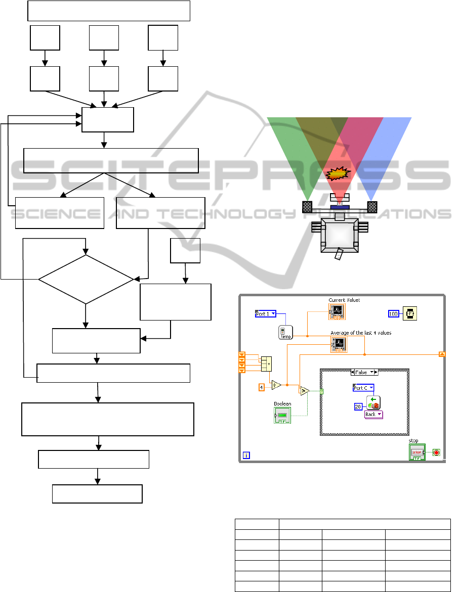
4 NAVIGATION STRATEGY
Since the sensors are fixed on the robot and the
movement of robot determines the direction of these
sensors, the vision of these sensors is limited to 45˚.
The sinusoidal movement, used for the navigation
strategy, turns the robot either 45˚ to the right or 45˚
to the left while searching for increasing levels of
light or heat. Control of this sinusoidal movement,
shown in Fig. 2, requires sensors with peripheral
vision of 180˚ in the direction of motion of the robot.
Figure 2: The visible range of sensors in a sinusoidal
movement.
ω
V
V
r
V
l
2b
θ
X
Z
DIRECTIONOFMOTION
FireDetectionRobotNavigationUsingModifiedVotingLogic
141

In order to cover 180˚ in the direction of motion it
was chosen to use a scanning approach such that, as
the robot travels in a straight line, the sensors cover
the area surrounding it.
The speed of the robot is 0.3 m/s at 100%
voltage input. The voltage can be modified in the
range from 0% to 200% to change speeds. The
sampling rate for the sensors is 10 times a second. A
sine wave, of given amplitude, had to be selected to
optimize the distance traveled, area scanned and
time elapsed to complete one cycle (Fig. 3).
The distance covered by the robot is directly
proportional to the amplitude of the sine curve path
chosen by the programmer. In a sine curve with
amplitude of 1, the length of a sine curve is 2.63π.
Depending on the requirements, the amplitude and
frequency can be chosen by the programmer. If there
is a need to scan a wider area, the amplitude can be
changed to a different value.
Figure 3: LabVIEW Virtual Instrument (VI) for sinusoidal
movement of the robot ending as a given high level of
light intensity is reached.
5 VOTING LOGIC APPROACH
5.1 Confidence Level
Confidence level is defined as the degree of
matching of the input signal to the features of an
ideal target, signal to interference ratio or number of
predefined features that are matched to the sensor
reading with the input signal. Here A
1
is denoted as
low confidence, A
2
and A
3
are denoted as medium
and high confidence levels for the sensor A,
respectively.
The number of confidence levels required for a
sensor is function of the number of sensors in the
system and the ease with which it is possible to
correlate target recognition features, extracted from
the sensor data, with distinct confidence levels. If
more confidence levels are available, the easier it is
to develop combinations of detection modes that
meet system detection and false-alarm probability
requirements under wide-ranging operating
conditions.
5.2 Voting Logic Sensor Fusion
As evident from the name, voting logic fusion fuses
the data of multiple sensors and based on the
information and confidence levels of these inputs
from the sensors, decision making is carried out
(Fig. 4). Voting logic fusion has many advantages
over single sensor based readings, used in series or
parallel. It provides a great deterrence against false
alarms, not compromising on the ability to detect
suppressed targets in a noisy environment. It may be
preferable technique to detect, classify and track
objects when multiple sensors are used.
Since one sensor, the ultrasonic sensor, is mainly
used for detection and avoidance of obstacles, it
does not need to be part of voting logic to declare
the presence of a fire (Fig. 5).Rather it would work
independently of the other sensors (Fig. 4). The
priority level for the sensor output is very high. As
the obstacle avoidance is very important to keep the
robot moving, the increasing gradient direction is
used for this purpose.
5.3 Modified Voting Logic
A fire declaration is only possible in the current
circumstances when the light readings above
threshold and the temperature above a certain level
are available. The probability of fire diminishes if
the light sensors are providing a reading that is
higher but the robot does not detect elevated
temperatures (Fig. 6). The robot may reach close to
the target where, due to robot geometry, the light
sensors may not give a reading that falls in any
confidence level given that the robot reached the
source. At that instance, the sensor A will give the
highest confidence level due to the temperature
present but, since the other sensors are not able to
sense it, voting logic will not declare a target based
on the output of just one sensor. At this point the
reading from the other sensors becomes irrelevant.
Normal voting logic does not keep this scenario
into account. In order to reach the point of interest
the robot has to follow any lead of increased light
only and will not declare the fire source until it
reaches a point where elevated temperatures are also
detected. To maximize the possibility of identifying
the target, an average of the previous four readings
is taken into account to linearize the readings hence
ICINCO2014-11thInternationalConferenceonInformaticsinControl,AutomationandRobotics
142
making the detection more reliable (Fig. 6). This is
achieved by introducing a while loop with shift
register in LabVIEW.
Figure 4: Fire declaration algorithm.
In the modified voting logic are incorporated
some of the attributes of parallel sensor combination
along with the conventional voting logic (Fig. 7).
The combinations of interest in fire detection with
two light sensors will only contain the ones that
include readings from the thermal infrared sensor.
Hence, the combination of the outputs containing the
two light sensors only has been excluded.
In the instance where light sensors are giving a
low confidence reading, or no reading, but the
temperature sensor is giving a very high confidence
reading, the fire incident is declared (Table 1). If the
thermal infrared sensor was defined as A and the
two light sensors were designated the letters B and
C, the voting logic described by the Venn diagram
shown in Fig. 7.
Fig. 8 shows LabVIEW implementation of
modified voting logic algorithm.
Figure 5: Possible combinations of sensor readings.
Figure 6: Single sensor based increasing gradient tracking
in LabVIEW implementation.
Table 1: Sensors and confidence levels.
Mode Sensors and Confidence Levels
A B C
ABC A
2
B
2
C
2
ABC A
3
B
1
C
1
AB A
2
B
3
-
AC A
2
- C
3
A A
4
- -
A B
C
D
W
A
W
B
W
C
Σ W
Voting Logic Rule (Fig. 8)
Low
Confidence Level
Threshold
Move to Source
Increased Gradient
(
Fi
g
. 6
)
Compare sensor readings, follow
increasing gradient
Maximum Gradient
Detect / Avoid
obstacles
High
Confidence Level
N
o
Sinusoidal Movement (Fig. 2 and 3)
Fire declaration
Yes
ABC
AC
AB
A
BC
FireDetectionRobotNavigationUsingModifiedVotingLogic
143
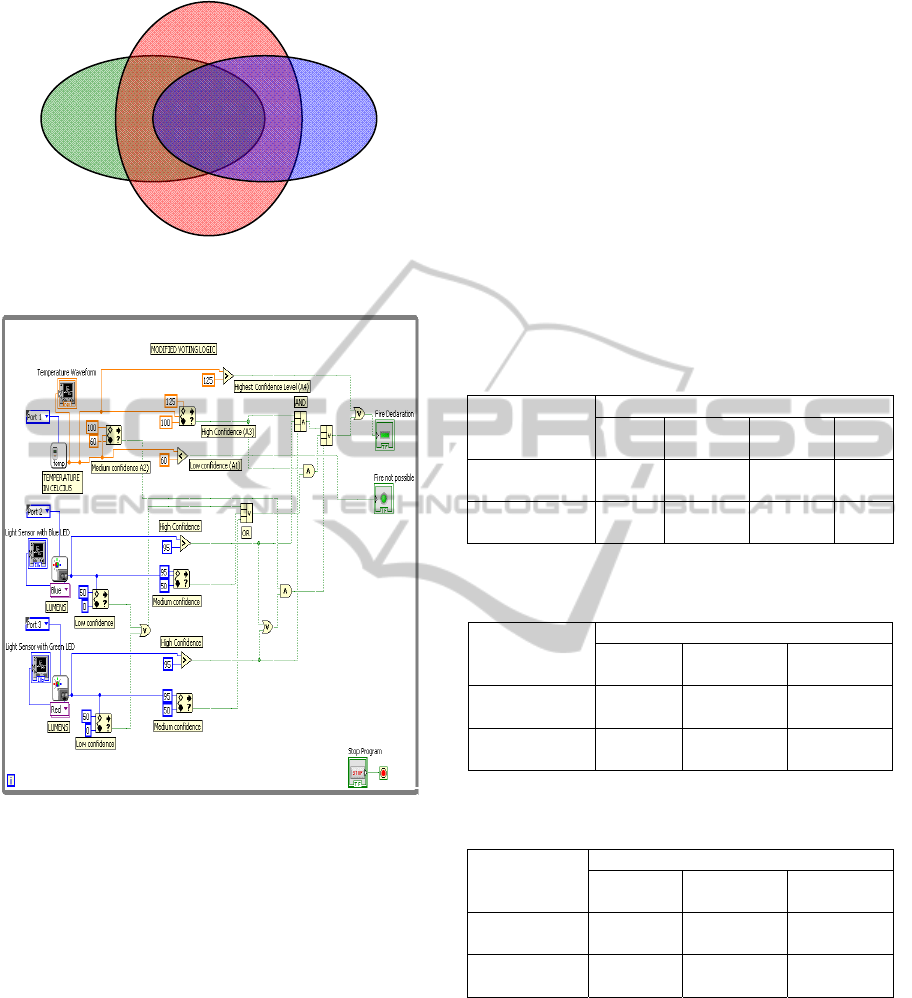
Figure 7: Combinations of interest in sensor outputs with
two light sensors and one thermal infrared sensor.
Figure 8: LabVIEW implementation of Modified Voting
Logic.
5.4 Detection Modes
In this section are presented the combinations of
sensor outputs that are able to declare a fire incident.
As more sensors detect different confidence levels,
the need to have higher confidence levels decreases.
Modes that contain two sensors are not required to
have the highest confidence levels as an intermediate
confidence level from all the sensors may be
sufficient to declare a fire incident. For the low
confidence level, however, all three sensors have to
be a part of the decision making process.
As mentioned in the last section, the voting logic
has to be modified in certain scenarios, so some
scenarios need to be excluded and some need to be
added. In the above mentioned case exclusions will
include any confidence levels of the sensors B and C
since they do not signify the presence of fire alone.
Also, if the highest confidence level from sensor A
is obtained, a fire incident is declared.
It can be noticed from Table 1 that there was no
mentioning of confidence level A
1
, as temperature
being a mandatory variable in fire detection, the
possibility of declaring fire is not considered when
confidence level A
1
is reported.
As the detection modes have been defined, now
it is possible to proceed with the derivation of
system detection and false-alarm probability using
the distributions presented in Table 2-4,with
assumed chosen for the illustration of the approach.
Table 2: Distribution of detections conditional
probabilities among sensor confidence levels for Sensor A.
Sensor
Confidence
Level
Sensor A
A
1
A
2
A
3
A
4
Distribution
of Detections
1000 700 500 400
Conditional
Probability
1.0 0.7 0.5 0.4
Table 3: Distribution of detections conditional
probabilities among sensor confidence levels for Sensor B.
Sensor
Confidence
Levels
Sensor B
B
1
B
2
B
3
Distribution
of Detections
100 500 300
Conditional
Probability
1.0 0.5 0.3
Table 4: Distribution of detections conditional
probabilities among sensor confidence levels for Sensor C.
Sensor
Confidence
Levels
Sensor C
C
1
C
2
C
3
Distribution
of Detections
100 500 300
Conditional
Probability
1.0 0.5 0.3
5.5 Fire Declaration Algorithm
As the detection modes have been defined, now it is
possible to proceed with derivation of system
detection and false-alarm probability
System P
d
= P
d
{A
2
B
2
C
2
or A
2
B
3
or A
2
C
3
or
A
3
B
1
C
1
or A
4
}
(6)
Applying the repeated Boolean algebra
expression for five detection modes a total of 4
A
B
C
ABC
AB AC
ICINCO2014-11thInternationalConferenceonInformaticsinControl,AutomationandRobotics
144
combinations are obtained
System P
d
= P
d
{A2}P
d
{B2}P
d
{C2} +
P
d
{A3}P
d
{B1}P
d
{C1} + P
d
{A2}P
d
{B3}
+ P
d
{A2}P
d
{C3} + P
d
{A4}
(7)
Similarly, the probability of false alarm
calculation for the system would be:
System P
fa
= P
fa
{A2}P
fa
{B2}P
fa
{C2} +
P
fa
{A3}P
fa
{B1}P
fa
{C1} + P
fa
{A2}P
fa
{B3} + P
fa
{A2}P
fa
{C3} + P
fa
{A4}
(8)
5.6 Confidence Levels Calculation
Mapping of the confidence-level space into the
sensor detection space is accomplished by
multiplying the inherent detection probability of the
sensor by the conditional probability that a particular
confidence level is satisfied given detection by the
sensor. Since the signal-to-interference ratio can
differ at each confidence level, the inherent
detection probability of the sensor can also be
different at each confidence level. Thus, the
probability P
d
{A
n
}, that Sensor A will detect a target
with confidence level A
n
, is
P
d
{A
n
} = P
d
'{A
n
} P{A
n
/detection} (9)
Where P
d
'{A
n
} is the inherent detection
probability calculated for confidence level n of
sensor A using the applicable signal-to-interference
ratio, false alarm probability, target fluctuation
characteristics, and number of samples integrated
and
P{A
n
/detection} is probability that detection
with confidence level A
n
occurs given a detection by
sensor A.
Similar process can be repeated to obtain the
false alarm probability of the system using P
fa
values. Using the data from Table 2-4, the results for
the detection probabilities for the sensor system are
shown in Table 5.
Table 5: System detection probabilities.
Detection probabilities for the suggested sensor system
Mode
Sensor A Sensor B Sensor C Mode P
d
A
2
B
2
C
2
0.58 0.35 0.35 0.07
A
3
B
1
C
1
0.45 0.4 0.4 0.07
A
2
B
3
0.58 0.26 0.15
A
2
C
3
0.58 0.26 0.15
A
4
0.39 0.39
System P
d
0.83
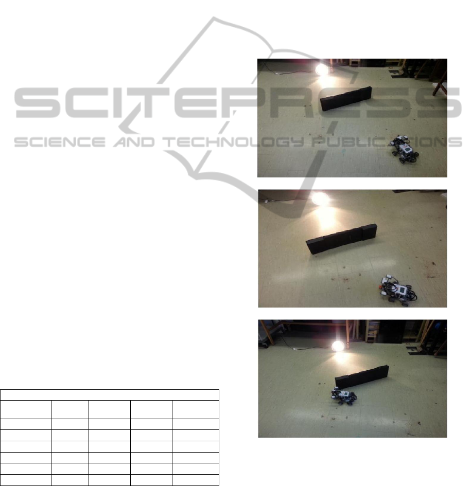
6 EXPERIMENTAL RESULTS
Experiments were performed on the robot NXT 2.0
for the validation of the algorithm. The results
showed a very high success rate of detecting the
source. In fact, the robot was able to identify the
light and heat source each time provided there was
no light reflecting off the surface of other objects.
Figure 9 presents the different steps in searching,
locating, obstacle avoidance, approaching the source
and declaring a fire incident.
The robot was able to identify the light and heat
source for different obstacle orientations and
configurations.
Figure 9: Robot starting behind an obstacle andmovingon
a sinusoidal path while detecting the heat source.
FireDetectionRobotNavigationUsingModifiedVotingLogic
145
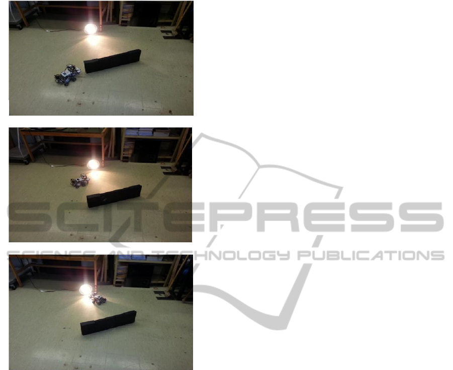
Figure 9: Robot starting behind an obstacle andmovingon
a sinusoidal path while detecting the heat source (cont.).
By limiting the detection mode of sensor A to the
2
nd
level for declaration, false alarm possibilities
have also decreased. There were few false alarms
during any experiment. The experiment were
performed a total of 30 times with 27 true
declarations. The success ratio was 90% in
declaration of the source.
7 CONCLUSIONS
Confidence level calculations and experimental
results show a consistency in recognizing and
declaring a fire source while minimizing the
possibility of a false alarm or non-declaration.
As a result of the adoption of single sensor
detection mode and also using single sensor non-
possibility mode, the accuracy of detecting a fire
increased. Also, this improvement was achieved
while not compromising on the ability to detect
suppressed or noisy targets.
Good source detection results were achieved by
the introduction of the sinusoidal movement
strategy. This increased the angle of peripheral
vision to 180˚ improved the detection probability by
helping the detection of a stronger source and, at the
same time, by bringing weaker sources into visible
range.
Introduction of comparison of stronger signals
while avoiding the obstacles resulted in a decrease
of the detection times.
The above combined improvements made the
detection system more reliable, more robust and
more accurate in tracking and in declaration of
indoor fires.
The system is also able to distinguish between a
reflected and direct signal coming from the source
based on the readings of different variables at the
approach of an obstacle.
REFERENCES
Karter, M. J. Jr., 2013, NFPA's Fire Loss in the United.
States during 2012, September.
Klein, L. A., 2004, Sensor and Data Fusion, a Tool for.
Information Assessment and Decision Making, SPIE.
Press, 2
nd
edition.
Zervas, E. et al., 2009, Multisensor Data Fusion for Fire.
Detection, Information Fusion, 12, pp. 150–159.
Khoon, T., 2012, Autonomous Fire Fighting Mobile.
Platform, IRIS 2012, International Symposium on.
Robotics and Intelligent Sensors, issue 4, pp. 1145 –
1153.
Viswanathan, R. and Varshney, P. K, 1997, Detection
with. Multiple Sensors: Part I – Fundamentals, Proc.
IEEE, vol85, issue 1.
Sasiadek, J. Z., 2002, Sensor Fusion, Annual Reviews in.
Control, IFAC Journal, No. 26, pp. 203-228.
Lilienthal, A. et al, 2006, Gas Source Tracing with a.
Mobile Robot Using an Adapted Moth Strategy, WSI,
University of Tubingen, Sand 1, 72074 Tubingen,
Germany.
David, C. T., 1982, A Re-Appraisal of Insect Flight.
Towards a Point Source of Wind-Borne Odour,
Journal of Chemical Ecology, issue 8, pp.1207–1215.
Ishida, H. et al., 1994. Study of Autonomous Mobile.
Sensing System for Localization of Odor Source
Using Gas Sensors and Anemometric Sensors, Sensors
and Actuator, vol. 45, pp. 153–157.
ICINCO2014-11thInternationalConferenceonInformaticsinControl,AutomationandRobotics
146
