Identification Technology of Mobile Phone Devices Using RFF

Saulius Japertas, Aurelijus Budnikas and Gedeiminas Činčikas

Department of Telecommunications, Kaunas university of technology, Studentų str. 50, Kaunas, Lithuania

Keywords: Rff, Wireless Devices Identification.

Abstract: The vulnerability of the device identifiers, such as IP and MAC addresses, IMEI and IMSI codes, etc.

creates threat to the information security, integrity and reliability. One of the solutions of this threat is usage

of Radio Frequency Fingerprinting (RFF) technology for identifying wireless devices based on their unique

radiation “fingerprint” as opposed to their addresses or codes. In this work identification problems of mobile

radio stations (from here in – mobile phones) are being analyzed and identification methodology for

identifying them based on the mathematical processing of front and rear fronts is proposed. All of this

provides new insight in the field of signal detection and identification, thus by using this method only the

original data is received. The purpose of this work is identification of a mobile phone, working on the DCS

(digital cellular service) frequency, based on the phone’s radiated signal time characteristics.

1 INTRODUCTION

The aim of this work is to explore the identification

possibilities of the mobile phone. Currently various

identification methods, such as identification of the

manufacturer’s model, according to the design of the

mobile phone, or identification according to the

physical and electrical parameters, or their entirety,

are being used. It is known, that each wireless device

has its own unique radiation characteristics (Danev

and Capkun, 2009), (Hall et al., 2003).

Identification of the wireless devices based on

the certain characteristics of the signal (phase, phase

and frequency errors, etc.) is proposed by other

authors (Hall et al., 2003), (Candore et al., 2009).

Technique to identify wireless device according

to its radiation characteristics is known as Radio

Frequency Fingerprinting. RFF are energy traces

that are left in the radio frequency spectrum. They

have certain characteristics that are emitted by every

transmitter. RFF allows to separate certain unique

characteristics that are radiated by every wireless

device even if several devices having the same

specifications are produced in the same plant (Danev

and Capkun, 2009), (Hall et al., 2003), (Danev et al.,

2012), (Danev et al., 2010). The essence of this

technique is that wireless devices are identified

according to the different radiation parameters such

as the phase characteristics of wireless device (Hall

et al., 2003), characteristics of various errors (Danev

et al., 2010), radiometric characteristics (Candore et

al., 2009). From these characteristics using various

mathematical models (such as Bayesian step change

detector (Hall et al., 2003) or Fisher linear

discriminant analysis (Danev and Capkun, 2009) the

certain parameters, that allow determining the

unique parameters of the transmitters, are calculated.

Identification is done by analyzing initial transient

signals.

By using RFF technique, identification system,

which can correctly determine the radio transmitter,

is formed. This system is an invaluable tool for

militaristic and civil purposes, where unauthorized

usage of electromagnetic specter is detected. It is

very useful to identify and localize the source of the

transmitted information. This system provides proof

that unsanctioned or illegal radio transmission is

being broadcasted (Shaw and Kinsner, 1997).

RFF technique is usually based on edge detection

and analysis of theirs various parameters, because

unique characteristics of every wireless device are

present within the boundary of these edges.

This technique is easily used to identify

transmitters, based on Bluetooth, 802.15.4 standard

(Danev and Capkun, 2009), WLAN 802.11 standard

(Danev and others, 2012), (Shaw and Kinsner,

1997), GSM (Zanetti and Lenders, 2012) and VHF

(Danev and others, 2012) standards.

Analysis of the aforementioned works shows that

practical usage of the identification techniques,

Japertas S., Budnikas A. and

Cin

cikas G..

Identiﬁcation Technology of Mobile Phone Devices Using RFF.

DOI: 10.5220/0005011800470052

In Proceedings of the 11th International Conference on Wireless Information Networks and Systems (WINSYS-2014), pages 47-52

ISBN: 978-989-758-047-5

 2014 SCITEPRESS (Science and Technology Publications, Lda.)

provided in these works, is met with certain

difficulties. The first problem is that it is quite

difficult to automate the identification process; the

second problem is the complexity of the

mathematical models, used in the identification

process (Danev and Capkun, 2009), (Hall et al.,

2003). In this work common math equations, which

can be easily implemented in the automated

identification system, are used. In this work, as well

as in many of the previous works, the identification

of the cell phone is based on the edge detection. In

this work is used a completely new methodology

based on discretization of the signals and description

on the shape of the edge by using mathematical

methods. In this paper we analyze the shape of the

signal amplitude in various aspects but do not

analyze characteristics of phase or errors.

2 EXPERIMENT AND

HARDWARE

This experiment was performed at Kaunas

University of Technology, Faculty of

Telecommunications, Radio Link laboratory. During

the experiment all mobile phones were functioning

on DCS frequency (1800MHz). All phones were

connected to the mobile network of the Tele2 Ltd.

(from herein after Tele2), one of the mobile

operators of Lithuania Republic. Algorithm of the

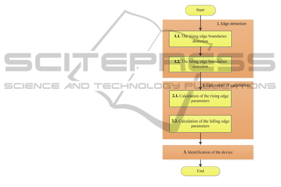
experiment is presented in Fig. 1.

This algorithm consists of three main parts.

1. Edge Detection. In the first part detection of

rising and falling edges is performed. This is

necessary to perform further calculations for

determining the edge curvature.

In this part the rising is detected. Firstly the

spectrum of the edge is calculated and 1ms length

part of the spectrum is taken. This part of the

spectrum is further discretized each 1µs. For each

discrete point the first derivative according to the

last discrete value is calculated. Rising edge

boundaries are detected according to the change of

this derivative.

After that boundaries of the falling edge are

detected according to the change of this derivative.

When change becomes significant enough, it is

considered, that the falling edge has begun. End of

the falling edge is considered as a point, when

change of derivative becomes low.

2. Calculation of Parameters. Calculation of

parameters is performed in the second part.

Calculation of the following rising edge

parameters is performed: the first and second

derivatives, curvature, slope coefficient. These

parameters are the central part of the work, since

they mathematically determine the shape of the

edge. If edge is a line, edge parameters of every cell

phone would be similar, but in reality they are

different.

3. Identification of the Device. In the third part

a matrix for identification of the device is created.

Figure 1: Algorithm of the experiment.

The following cell phones were tested: Nokia

X3, Nokia C3, Nokia 3600, Nokia 7260, two Nokia

6230i (further referred to as A and B), Samsung

E390.

During the work, spectrum analyzer

Rohde&Schwarz FSH8 was used. Its operating

frequency band is 9 kHz – 10 GHz. This device

ensures good sensitivity without additional amplifier

(up to – 141 dBm). Antenna used in this work was

omnidirectional and calibrated for 18700 MHz

frequency band.

During experiments in the laboratory, WLAN

networks were detected, but they did not interfere

with the experiments because their frequencies were

different (WLAN operates in 2400 MHz band and

experiments were performed in 1800 MHz band).

WINSYS2014-InternationalConferenceonWirelessInformationNetworksandSystems

Experiment was performed in strictly controlled

environment and on identical system settings.

During all experiments the same antenna, connector

cables and spectrum analyzer were used. To enhance

the transmitted signal and to avoid using additional

amplifying equipment we chose to use a small

distance between cell phone and spectrum analyzer

is 0.5 m. For each phone 80 measurements were

performed. Correlation coefficient of the

measurements was >95%, and error less than 8%.

Transmitted signal was initiated by call from the

mobile phone, thus monitored transmitting

frequency band was 1758-1782 MHz. Transmitted

signal frequency characteristics were collected from

3hr long calls by making a call each 2 minutes.

Results were collected on different days. No

significant differences were detected. Thus it can be

said that further experiments for certain band should

be easily performed. Stable conditions for all the cell

phones, which were used in the experiment, must be

assured. For the remaining part of the experiment a

certain frequency, in which all the following steps of

the experiment will be performed, is chosen. A 1765

MHz frequency was chosen, because signal

amplitude (strength) is strongest on this frequency.

3 RESULTS

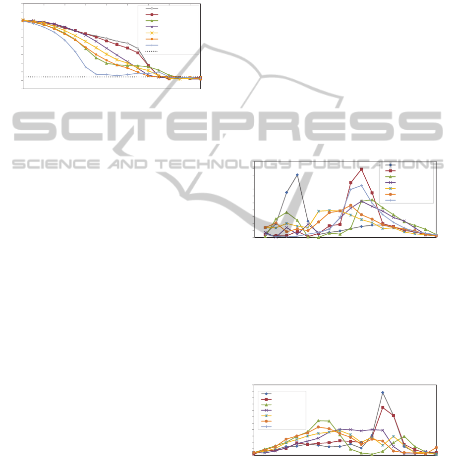
As shown by the experiments, rising and falling

edges of all cell phones (power vs time), even of the

same brand (Nokia 6230i A and B), were different

(Fig. 2, 3).

Theoretically, duration of the rising and falling

edges are not accurately determined (but maximum

duration of the edge can be 28 µs), thus it can be

different (Molisch, 2011). Result analysis clearly

shows that longest duration of the edge change was

17 µs (Fig. 2). Thus it was decided that rising edge

will be sampled for a period of 17µs with a sampling

time of 1µs.

By sampling signal in the time axis, we obtain

specific signal amplitudes for each sampling step. In

this case we chose to discretize signal each 1 µs.

Falling edge of the signal is shown in Fig. 3. As

in the case of the rising edge, falling edges of all 7

cell phones are shown next to each other. Maximum

duration of the edge change was 16 µs, but, to meet

the identical conditions, discretization period was set

to 17 µs.

Figure 2: Rising edge.

Figure 3: Falling edge.

Average amplitudes of all rising edge signals are

shown in Fig. 4. Also noise level is addressed here.

It is obvious, that edge shapes of individual cell

phones are different. We can clearly see differences

between different mobile phones: their uniformity,

curvature, etc. In example, cell phone “Nokia X3”

has extra clear and wide signal edge curve. During

the experiment this was one of the most visually

apparent differences between rising fronts, created

by sending signals from this call phone. On the other

hand rising edge of the “Nokia C3” cell phone is

below the noise level until approximately 7 µs, thus

we can conclude that the rising edge of this cell

phone is shortest as well as steepest. Also rising

edge on a “Nokia 3600” cell phone was particularly

interesting: it has clear directivity and breaking

points.

‐70

‐65

‐60

‐55

‐50

‐45

‐40

‐35

‐30

‐25

‐20

0246810121416

Power, dBm

Time, µs

(Nokia X3)

(Nokia C3)

(Nokia 3600)

(Nokia 7260)

(Nokia 6230i A)

(Nokia 6230i B)

(Samsung E390)

Noise

Figure 4: Power of the rising edge of the cell phone signal

as function of time (averages).

Falling edges of 7 cell phones are shown in

Fig. 5. As we can see from the charts, as in the case

IdentificationTechnologyofMobilePhoneDevicesUsingRFF

of rising edge, “Nokia X3” has a clear breaking

point. Signal curve of cell phone “Nokia S3” is very

similar to the curve of “Nokia X3”.

Experiment results of two identical cell phones

“Nokia 6230i” should be specifically mentioned.

The first call phone was marked with letter “A”,

second – with letter “B”.

‐70

‐65

‐60

‐55

‐50

‐45

‐40

‐35

‐30

‐25

‐20

0246810121416

Power, dBm

Time, µs

(Nokia X3)

(Nokia C3)

(Nokia 3600)

(Nokia 7260)

(Nokia 6230i A)

(Nokia 6230i B)

(Samsung E390)

Noise

Figure 5: Power of the falling edge of the cell phone signal

as function of time (averages).

In references (Danev et al., 2010), (Shaw and

Kinsner, 1997) it is noted, that signal characteristics

of the cell phones of identical manufacturer and

brand should be quite similar or have slight

differences.

As we can see from Fig. 4 and 5, the difference

between such cell phones is not too big, but it is

quite significant. It will be later shown that this

difference, after mathematical processing, will

become much more apparent. Falling edge of the

cell phone “Nokia 3600”, as its rising edge, has an

apparent directional variation and several breaking

points during a 17 µs period. On the other hand

falling edge of the “Samsung E90” rapidly falls

down close to noise level but, as shown in the

diagram, later rises slightly after a rapid fall.

Duration of the falling edges is relatively slightly

shorter than the duration of the rising edges because

falling edges of most mobile phones drop down to

noise level after 14 -15 µs.

From Fig. 4 and 5 we can form an opinion that

GSM packets of a specific tested cell phone have

visually similar rising and falling edges. In example,

looking at “Nokia 3600” transmitted signal edges it

is visually apparent that shape of the falling edge is

similar to the shape of the rising edge – breaking

points and directional variations are clearly visible in

both rising and falling edges. The same applies to

both “Nokia 6230i” cell phones marked by orange

and yellow colors. It has to be said that in the cases

of other cell phones, i.e. “Samsung E930”, rising

edge is different from the falling edge. Despite that

later mathematical processing showed, that these

fronts are not their own “mirror images” according

to their shape.

As we can see from Fig. 2-5, rising and falling edges

of each phone are curves and they can be described

by the 1st and 2nd order derivatives, edge curvature

and edge slope coefficient.

The First Derivative. It is known that the first

derivative shows the speed of the functions quantity

change. Signal edges, obtained during this

experiment can be described by derivative, showing

the speed of the amplitude change. The higher this

number, the greater the change in comparison with

the previous value. As the derivative approaches

zero, the edge of the signal becomes straighter (the

form change stops). By using the results of the first

derivative we can detect the borders of the signal

edge, used to assure identical conditions to all tested

cell phones.

A combined chart of all 7 tested cell phones first

derivatives (in relative units) of the rising edge is

shown in Fig. 6.

0 2 4 6 8 10 12 14 16

The first derivative, r.u.

Time, µs

Nokia X3

Nokia C3

Nokia 3600

Nokia 7260

Nokia 6230i A

Nokia 6230i B

Samsung E390

Figure 6: The first derivative of the rising edge.

As we can see from the combined chart, the first

derivatives of each cell phone are different. It is

most visible with the cell phones “Nokia X3” and

“Nokia C3”. The first derivatives of other cell

phones are slightly lower, which means that the

changes of certain intervals are lower. A combined

chart of all 7 tested cell phones first derivatives of

the falling edge is shown in Fig. 7.

0246810121416

The first derivative, r.u.

Time, µs

Nokia X3

Nokia C3

Nokia 3600

Nokia 7260

Nokia 6230i A

Nokia 6230i B

Samsung E390

Figure 7: The first derivative of the falling edge.

Thus the charts of the first derivatives shows the

intensity of the function change over time. The

WINSYS2014-InternationalConferenceonWirelessInformationNetworksandSystems

higher the intensity of this change results in higher

change of the amplitude and more apparent edge

curvature. In Fig. 6 and 7 we can see that derivatives

of the cell phones “Nokia X3” and “Nokia C3” are

the highest and in Fig. 4 and 5 we can see that the

edges of these phones are distinguished by their

individuality.

The Second Derivative. The second derivative

shows if a function has a breaking point (a point

where it’s direction changes) in the function change

interval. Existence of the breaking point is

considered the point where function of the second

derivative crosses zero axis. Results of the second

derivative of the rising edge are shown in Fig. 8 and

of the falling edge in Fig. 9.

Thus in these figures we can see a clear

differences between the second derivatives of the

edges of each phone. Changes of the second

derivative are especially clear in the case of a

“Nokia X3” with highest change being at 5 µs. Also

the value of the second derivative is big for the cell

phone “Nokia C3”. It is also apparent that the

second derivatives of various phones cross the y = 0

axis different number of times: 3 times for “Nokia

X3”, 4 for “Nokia C3” (Fig. 8). The time of these

crossings is different in each case as well.

‐7

‐6

‐5

‐4

‐3

‐2

‐1

0246810121416

The second derivative, r.u.

Time, µs

Nokia X3

Nokia C3

Nokia 3600

Nokia 7260

Nokia 6230i A

Nokia 6230i B

Samsung E390

Figure 8: The second derivative of the rising edge.

‐6

‐5

‐4

‐3

‐2

‐1

0 2 4 6 8 10 12 14 16

The second derivative, r.u.

Time, µs

Nokia X3

Nokia C3

Nokia 3600

Nokia 7260

Nokia 6230i A

Nokia 6230i B

Samsung E390

Figure 9: The second derivative of the falling edge.

The second derivatives of all phones first points

are not large, since as it is shown in Fig. 6, the

shapes of falling edges for all phones are bending

down slowly and do not change the direction of

approximately up to 10 s time interval. In this case,

mobile phone “Samsung E390” stands out, as the

second derivative here has a breaking point and

changes sign already at 7 µs. The highest points of

the second derivative are also at 12 µs of falling

edges curves for “Nokia X3” and “Nokia C3”

mobile phones. Curvature of these phones has been

observed at the first derivative as well.

Calculated the second derivatives of two mobile

phone signals for the same model “Nokia 6230i”

visually looks similar. However, under the analysis

it can be seen a sufficient difference. This difference

apparently could be influenced by a wider shape

(form) of mobile phone falling edge (Fig. 5).

Curvature and slope coefficient. The curvature K

of the curve can be calculated using the equation (1)

(Curvature definition, 2010):

1(')













(1)

where

y and ''y is first-and second-order

function's (in our case it is power) derivatives

respectively.

Slope coefficient b is an expression showing the

dependence of average of the random variable on the

other variable (several variables). Slope coefficient

is calculated using equation (2). It shows how the

signal edge steeply arises (or descends) (SLOPE

function definition):

()( )

()

xy y









(2)

where x (in our case it is time) and y (in our case

it is power) are argument and function respectively.

Curvature is calculated using the first and second

derivatives. The curvature is calculated at each point

of the sampling and shows sharpness of the curve is

bending. In this case, the greater the curvature at that

point is the stronger deformation is observed. All

that is well seen by looking at the waveform.

Meanwhile, the curvature is less, the shape of signal

edge is straighter and smoother. Curvature is equal

to 0 if the waveform is straight. The curvature of

rising and falling edges are shown in Fig. 10. As it

can be seen from this figure, curvatures of different

edges are significantly different. “Nokia 3600” and

“Nokia X3” have large curvatures for the rising

edge, while phone model „Samsung E390“has the

largest curvature of falling edge. Curvatures of the

two mobile phones model of “Nokia 6230i” are also

clearly different.

IdentificationTechnologyofMobilePhoneDevicesUsingRFF

As mentioned above, the slope coefficient will

show the signal edge slope. This means that the

slope coefficient is higher, the mobile phone edge is

steeper. Slope coefficient is calculated from all

sampling points, i.e. using 18 points. In Fig. 11 we

can see that the lowest slope coefficient is in the

case of mobile phone “Nokia X3” raising edge.

Meanwhile, the highest slope coefficient is in the

cases of “Nokia C3” and “Samsung E390"signal

rising edges.

Thus, the presented results have shown that it is

possible to describe the rising and falling edges of

mobile phone transmitting signals using simple

mathematical categories. Following the creation of

corresponding matrix of such data, identification of

the mobile phones should be possible. The greater

number of parameters in a matrix, the higher

probability of the mobile phone identification.

However, the assessment of a larger number of

parameters and the formation of the matrix will be

done in subsequent works.

0,00

0,10

0,20

0,30

0,40

0,50

0,60

NokiaX3 NokiaC3 Nokia

3600

Nokia

7260

Nokia

6230(A)

Nokia

6230(B)

Samsung

E390

Averagecurvature,r.u.

Mobilephonemodel

RisingEdge

FallingEdge

Figure 10: Edges average curvature dependence on the

mobile phone model.

0,0

0,5

1,0

1,5

2,0

2,5

3,0

NokiaX3 NokiaC3 Nokia

3600

Nokia

7260

Nokia

6230(A)

Nokia

6230(B)

Samsung

E390

Slopecoefficient,r.u.

Mobilephonemodel

RisingEdge

FallingEdge

Figure 11: Edges slope coefficient dependence on the

mobile phone model.

Some issues are planned for further works: to

describe accurately identification algorithm for

mobile station, perform measurements with the

mobile station in further distance from the spectrum

analyzer, perform measurements with other wireless

devices.

4 CONCLUSIONS

Measurements have shown that rising and falling

edges of transmitted signal for different mobile

phones vary even when the phone models are the

same.

The experimental results of measurement are

estimated to not exceed 8% of the error; the

correlation coefficient of measurement results for

each model is > 0.95.

New digital wireless device identification

method based on assessment of signals rising and

falling edges form has been proposed. This method

is based on the calculation of rising and falling edges

parameters using mathematical methods – the first

and second derivatives, curvature and slope

coefficient.

Number of identification parameters will be

increased and the algorithm for the identification of

devices will be proposed in further works.

REFERENCES

Danev B., Capkun S., 2009. Transient-based Identification

of Wireless Sensor Nodes. IPSN’09, San Francisco,

California, USA.

Hall J., Barbeau M., Kranakis E., 2003. Proceedings of

IASTED International Conference on Wireless and

Optical Commnications (WOC), Banff, Alberta.

Candore A., Kocabas O., Koushanfar F., 2009. Robust

Stable Radiometric Fingerprinting for Wireless

Devices. IEEE International Workshop on Hardware-

Oriented Security and Trust, San Francisco, CA, USA.

Danev B., Zanetti D., Capkun S., 2012. On Physical-layer

Identification of Wireless Devices. ACM Computing

Surveys (CSUR).

Danev B., Luecken H., Capkun S., 2010. Attacks on

Physical-layer Identification. WiSec '10 Proceedings

of the third ACM conference on Wireless network

security.

Shaw D., Kinsner W., 1997. Multifractal Modelling of

Radio Transmitter Transients for Classification.

WESCANEX 97: Communications, Power and

Computing. Conference Proceedings., IEEE

Zanetti D., Lenders V., 2012. Exploring the Physical-layer

Identification of GSM Devices.

Molisch A. F., 2011. Wireless Communications, John

Wiley and Sons, 2nd Edition.

Curvature. Definitions and Examples. College of Science

and Mathematics 2010. URL: http://science.

kennesaw.edu/~plaval/math2203/curvature.pdf

SLOPE function definition on Microsoft Office support

resources. URL: http://office.microsoft.com/en-

au/excel-help/slope-HP005209264.aspx

WINSYS2014-InternationalConferenceonWirelessInformationNetworksandSystems