
Digital Self-tuning Control for Pressure Process
Gediminas Liaucius and Vytautas Kaminskas
Department of Systems Analysis, Vytautas Magnus University, Vileikos Str. 8, LT-44404 Kaunas, Lithuania
Keywords: Self-tuning PID Control, Closed-loop Parameters and Sampling Period Optimization, Predictor-based Self-
tuning Control with Constraints, Pressure Process.
Abstract: Two digital control systems - Self-tuning PID (Proportional-Integral-Derivative) Control and Predictor-
based self-tuning control with constraints - for the continuous-time pressure process control are presented in
this paper. The digital self-tuning PID control with optimization of closed-loop parameters and sampling
period is proposed. The multidimensional optimization problem of closed-loop parameters and sampling
period is solved by subcomponent search method that enables dividing the problem to one-dimensional
optimization problems. The golden section search is adjusted to solve those – one-dimensional -
optimization problems. The predictor-based self-tuning control with constraints is adapted for both
minimum-phase and nonminimum-phase process models. The control quality of pressure process of both
control systems has been experimentally investigated. The results of experimental analysis demonstrate that
the digital self-tuning PID control with optimization is more efficient as compared to predictive-based self-
tuning control with constraints for pressure process.
1 INTRODUCTION
At present, various physical nature processes are still
continuous-time processes, but are frequently
controlled by digital controllers (Isermann, 1991;
Åström and Wittenmark, 1997; Bobál, et al, 2005).
The digital PID (proportional-integral-derivative)
control laws are the most common for such
processes (Åström and Hagglund, 1995; 2001;
Levine 1999). The PID controllers are so widely
used for its easiness to apply and generally provides
sufficient control quality if it is properly tuned.
For the digital PID control based on digital self-
tuning PID controllers the selection of suitable
closed-loop parameters (Vu, et al, 2007; Kosorus,
et al, 2012) and proper sampling period (Boucher,
et al, 1989; Isermann, 1991; Åström and
Wittenmark, 1997; Levine, 2011) is substantial since
directly influences the control quality of the process.
Furthermore, the determination of closed-loop
parameters and sampling period is not
straightforward, at the design stage of the control.
The digital self-tuning PID control system with
on-line identification and optimization of closed-
loop parameters and sampling period is developed
for pressure process control (Liaucius, et al, 2011;
Liaucius and Kaminskas, 2012a) in this paper.
As an alternative to self-tuning PID control for
pressure process, the predictor-based self-tuning
control with constraints (Kaminskas, 2007) is
analysed. This control method has been modified for
both minimum-phase and nonminimum-phase
process models. The results of experimental analysis
of both control approaches are presented.
2 THE PRESSURE PROCESS
The scheme of pressure process is depicted in
Figure 1.
The process consists of four main components:
combined air inlet and outlet tanks, two air chambers
and two tubes with balls in them. The air from the
inlet tank flows to air channels through air chambers
and leaves the equipment through the upper outlet
tank. The distance to balls is measured using
ultrasound distance sensors. The fans are used to
create pressure in the air channels in order to lift the
balls in tubes. The air chambers are utilized for the
purpose to stabilize oscillations of the pressure in
each tube. The momentum of the fan, the inductance
of the fan motor, air turbulence in the tube leads to
complex physics governing ball behaviour. Slightly
different weights of the balls and the location of the
612
Liaucius G. and Kaminskas V..
Digital Self-tuning Control for Pressure Process.
DOI: 10.5220/0005012106120619
In Proceedings of the 11th International Conference on Informatics in Control, Automation and Robotics (ICINCO-2014), pages 612-619
ISBN: 978-989-758-039-0
Copyright
c
2014 SCITEPRESS (Science and Technology Publications, Lda.)
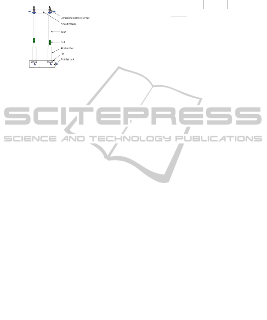
air feeding vent additionally impact the behaviour of
ball in the tubes.
Figure 1: The scheme of the pressure process.
The control signals (inputs) of the process are the
voltage values for each fan from the range 0 to 10V.
The intermediate values of voltage affect the power
of the fan proportionately. The control responses
(outputs) are the distances between the balls and the
bottom of their tubes from the range 20 to 90 in
centimetres. The control problem is to regulate the
speed of the fan supplying the air into the tube so as
to keep the ball suspended at some pre-determined
level in the tube.
3 SELF-TUNING PID CONTROL
WITH OPTIMIZATION
The mathematical model of the process is necessary
in order to design the digital PID control system
with on-line identification. Each tube of the process
is defined by discrete linear second order difference
equations, i.e.
,
)()(1)()(1)( i
t
i
t
ii
t
i
uzByzA
(1)
,
,1
2
)(
2
1
)(
1
1)(
2
)(
2
1
)(
1
1)(
zbzbzB
zazazA
ii
i
ii
i
(2)
where
)(
1)(
zA
i
, )(
1)(
zB
i
are the model polynomials,
2,1i
is the number of the tube of pressure process,
)(
0
)(
)(
tTyy
i
i
t
,
)(
0
)(
)(
tTuu
i
i
t
- output and input
signals with sampling period
0
T
respectively,
)(i
t
- a
white noise of the
thi
tube with a zero mean and
finite variance and
1
z
is the backward-shift operator
(
)(
1
)(
1
i
t
i
t
yyz
).
Unknown model parameters of the
thi
tube
,,,,
)(
2
)(
1
)(
2
)(
1
)(
iiii
Ti
bbaa
(3)
are estimated by recursive least squares algorithm
with forgetting factor (Liaucius and Kaminskas,
2012a)
otherwise
C
zeif
i
t
i
t
i
t
i
t
i
t
i
j
i
e
i
t
i
t
i
t
,
ˆ
1
ˆ
1or,
ˆ
ˆ
)(
)(
)(
1
)(
)(
1
)(
)()(
)(
1
)(
(4)
,
ˆ
ˆ
,
,,,,
)(
1
)(
1
)()(
)(
1
)()(
1
)(
)(
2
)(
1
)(
2
)(
1
)(
i
t
Ti
t
i
t
i
t
i
t
i
t
Ti
t
i
t
i
t
i
t
i
t
i
t
Ti
t
y
C
uuyy
(5)
0,
0,
ˆ
)(
)(
1
)()(
)(
)(
1
)(
1
)(
1
)(
1
)(
1
)(
1
)(
i
t
i
t
i
t
i
t
i
t
i
t
i
t
Ti
t
i
t
i
t
i
t
i
t
ifC
if
CC
C
C
(6)
,
1
)(
1
)(
)()(
i
t
i
t
i
t
i
t
(7)
,
)(*)()( i
t
i
t
i
t
yye
(8)
where
)(i
t
e
is the control error,
)(i
e
- a constant that
defines the admissible interval of control error
)(i
t
e
and
,
)(i
j
z
2,1j
are the roots of polynomial
)(
ˆ
1
)(
zA
i
t
and
*)(i
t
y
is a reference signal of the
thi
tube.
Applying on-line identification algorithm (4), the
estimates of model parameters are updated only if
the value of
)(i
t
e
is outside of the admissible interval
defined by
)(i
e
and the current on-line model is
stable.
The results of on-line identification of models
are used to the digital self-tuning PID controllers
(Ortega and Kelly, 1984; Bobál, et al, 2005), which
are defined as follows:
,
)(1)()()()(1)( i
t
i
t
i
t
i
t
i
t
i
t
yzReuzS
(9)
,
,11
2
)(
2
1
)(
2
)(
0
)(
0
1
)(
)(
11
)(
zrzrrrzR
zzS
i
t
i
t
i
t
i
t
i
t
i
t
i
t
(10)
where
)(i
t
e
is the control error (8),
,
)(i
t
S
)(i
t
R
are the
polynomials and
)(
2
)(
0
)()(
,,,
i
t
i
t
i
t
i
t
rr
are the parameters
of the controller of the
thi
tube that are calculated
by expressions
,
ˆ
ˆ
1
ˆ
1
)(
0
)(
1
)(
)(
1
)(
1
)(
1
)(
i
t
i
t
i
t
i
t
i
i
t
i
t
rbad
b
(11)
,
ˆ
ˆ
ˆ
ˆ
ˆ
ˆ
,
ˆ
ˆ
)(
2
)(
2
)(
2
)(
1
)(
2
)(
1
)(
2
)(
0
)(
2
)(
2
)(
2
)(
i
t
i
t
i
t
i
t
i
t
i
t
i
t
i
t
i
t
i
t
i
t
i
t
b
a
a
a
b
b
rr
a
b
r
(12)
,
ˆ
ˆ
1
ˆ
ˆ
,
ˆ
ˆˆˆ
ˆ
ˆ
ˆ
2
)(
1
)(
2
)(
1
2
)(
2
)(
2
)(
2
)(
2
)(
2
)(
1
)(
2
)(
1
)(
1
)(
2
)(
2
)(
2
i
t
i
t
i
t
i
t
i
t
i
t
i
t
i
t
i
t
i
t
i
t
i
t
i
t
i
t
i
t
badbar
adbbbabar
(13)
DigitalSelf-tuningControlforPressureProcess
613
,
ˆˆ
ˆ
ˆˆ
ˆ
ˆˆ
2
)(
2
2
)(
1
)(
2
)(
2
)(
1
)(
1
)(
2
)(
1
)(
2
)(
2
)(
2
i
t
i
t
i
t
i
t
i
t
i
t
i
t
i
t
i
t
i
t
i
t
bbabbabb
rr
r
(14)
which are obtained by solving the system
)(
4
)(
2
)(
3
)(
2
)(
1
)(
2
)(
1
)(
1
)(
)(
)(
2
)(
0
)(
2
)(
2
)(
1
)(
2
)(
1
)(
2
)(
2
)(
1
)(
2
)(
1
)(
1
)(
2
)(
1
)(
1
ˆ
ˆˆ
ˆ
1
ˆ
0
ˆ
0
ˆˆ
0
ˆˆˆ
1
ˆ
ˆˆˆˆ
1
ˆ
0
ˆ
i
i
t
i
i
t
i
t
i
i
t
i
i
t
i
t
i
t
i
t
i
t
i
t
i
t
i
t
i
t
i
t
i
t
i
t
i
t
i
t
i
t
i
t
i
t
i
t
d
ad
aad
ad
r
r
ab
aabbb
abbbb
bb
(15)
where
,0,2exp
,
1,1cosexp2
1,1cosexp2
)(
4
)(
3
0
)(
2
2
00
2
00
)(
1
iii
i
ddTd
ifTT
ifTT
d
(16)
is the natural frequency of oscillation,
is the
damping factor of characteristic equation of
continuous-time closed-loop system
.02
22
ss
(17)
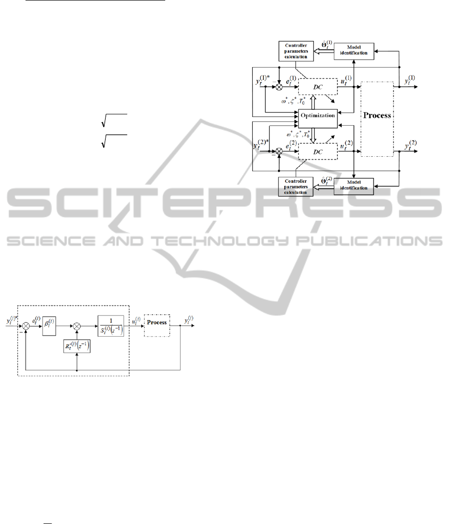
The scheme of the digital PID controller is depicted
in Figure 2. Such structure of PID controller is more
effective as compared to the structure of
conventional PID controller for pressure process
control (Liaucius, et al, 2011).
Figure 2: The scheme of the digital PID controller.
The required control response of control system with
digital self-tuning PID controllers can be achieved
by the selection of proper closed-loop parameters (
,
) and sampling period (
0
T
). Therefore, is
reasonable to find such values (
*
0
**
,, T
) of these
parameters that minimize control quality criterion
,
min
,,:,,
0
,,
0
*
0
**
T
TQT
(18)
},
{
1
,,
2
)2(
1
*)2(
2
)1(
1
)1(
1
2
)2(*)2(
2
)1(*)1(
0
t
t
t
t
N
t
tttt
uuuu
yyyy
N
TQ
(19)
where
N
is the number of observations,
*)(i
t
y
is the
reference signal of the
thi
tube,
0
is a weight
coefficient. The criterion consists of two parts: the
first part estimates the variance of control error of
each tube, the second - characterizes the variance of
control signal change of each tube.
The scheme of the digital self-tuning control of
the pressure process is depicted in Figure 3.
Figure 3: The scheme of the digital self-tuning control of
the pressure process.
The optimization problem (18) is solved as follows.
The optimal sampling period
*
0
T
is obtained by
,
min
:
0
,,
0
*
0
T
T
TJT
(20)
.,,min
0
,
0
TQTJ
T
(21)
The optimal closed-loop parameters
**
,
are
obtained by
.
min
,,:,
,
*
0
**
TQ
(22)
In order to solve optimization problem of (20), a
technique of one dimensional search is used. The
most popular algorithms of this technique are golden
section and quadratic interpolation (Kaminskas,
1982). The results of experimental analysis
(Liaucius and Kaminskas, 2012b) showed that
golden section algorithm for pressure process is
more effective.
Golden section algorithm is related with an
initial uncertainty interval
,,0,
max00401
TTT
(23)
reduction to the interval
,,,
0
)(
01
)(
04
)(
04
)(
01
TTTifTT
LLLL
(24)
where its length is not longer than desired
0
T
and
with a function (21) minimum inside. For this
purpose, two new values of sampling period
0
T
are
chosen by
ICINCO2014-11thInternationalConferenceonInformaticsinControl,AutomationandRobotics
614

Ll
TTTT
TTTT
llll
llll
,,2,1,
618.0
382.0
)(
01
)(
01
)(
04
)(
03
)(
01
)(
01
)(
04
)(
02
(25)
in the search procedure and a new uncertainty
interval is then defined by the rule
.
,,,
,,,
)(
04
)(
02
)1(
04
)1(
01
)(
03
)(
02
)(
03
)(
01
)1(
04
)1(
01
otherwiseTTTT
TJTJifTTTT
llll
l
T
l
T
llll
(26)
Then the optimal sampling period
*
0
T
is obtained by
.
,
,
)1(
03
1(
03
1(
02
)1(
02
*
0
otherwiseT
TJTJifT
T
L
L
T
L
T
L
(27)
The subcomponent optimization method
(Kaminskas, 1982) is applied to solve the
optimization problem of (21):
,2,1,
min:
min:
)(
)(
j
J
J
j
j
(28)
where
,
,,
,,
)1(
0
)(
)1(
0
)1(
l
j
l
j
TQJ
TQJ
(29)
)1(
0
l
T
is a
0
T
value, obtained by golden section
algorithm, where the new value of (21) must be
calculated, i.e.:
.
,
,
)1(
03
)(
03
)(
02
)1(
02
)1(
0
otherwiseT
TJTJifT
T
l
l
T
l
T
l
l
(30)
Each of the optimization problems (28) are solved
by golden section search analogously to (23)-(27).
4 PREDICTOR-BASED SELF-
TUNING CONTROL WITH
CONSTRAINTS
Since the pressure process is defined by the model
(1)-(2), the control law of predictor-based self-
tuning controller with constraints (Kaminskas, 2007)
for the
thi
tube is described by equations
,
,
~
,,max
~
,
~
,,min
)(
1
)()(
)(
min
)(
)(
1
)(
1
)()()(
max
)(
1
otherwiseuuu
uuifuuu
u
i
t
i
t
i
t
i
i
t
i
t
i
t
i
t
i
t
i
i
t
(31)
,
~
~
*)(
1
)(1)(
)(
1
1)(
i
t
i
t
i
t
i
t
i
t
zyyzLuzB
(32)
,
~~~
~
2
)(
2
1
)(
1
)(
0
1)(
zbzbbzB
i
t
i
t
i
t
i
t
(33)
,
ˆˆˆˆ
1
)(
2
)(
1
)(
2
2
)(
1
1
)(
1
)(
0
1)(
zaaaa
zllzL
i
t
i
t
i
t
i
t
i
t
i
t
i
t
(34)
where
,
1
ˆ
/
ˆ
1
ˆ
,
ˆ
ˆ
1
ˆ
/
ˆ
1
ˆ
,
ˆ
ˆ
1
ˆ
/
ˆ
1
ˆ
,
ˆ
1
ˆ
/
ˆ
1
ˆ
,
ˆ
~
)(
1
)(
2
)(
1
)(
2
)(
1
)(
1
)(
2
)(
1
)(
1
)(
1
)(
1
)(
2
)(
1
)(
2
)(
1
)(
2
)(
1
)(
1
)(
0
i
t
i
t
i
t
i
t
i
t
i
t
i
t
i
t
i
t
i
t
i
t
i
t
i
t
i
t
i
t
i
t
i
t
i
t
i
t
bbandaifba
bbandaifba
bbandaifb
bbandaifb
b
(35)
,
1
ˆ
/
ˆ
1
ˆ
,
ˆ
ˆ
ˆ
1
ˆ
/
ˆ
1
ˆ
,
ˆ
ˆ
ˆ
1
ˆ
/
ˆ
1
ˆ
,
ˆ
ˆ
ˆ
1
ˆ
/
ˆ
1
ˆ
,
ˆ
ˆ
ˆ
~
)(
1
)(
2
)(
1
)(
1
)(
1
)(
2
)(
1
)(
2
)(
1
)(
2
)(
1
)(
1
)(
1
)(
2
)(
1
)(
2
)(
1
)(
1
)(
1
)(
2
)(
1
)(
1
)(
1
)(
2
)(
1
i
t
i
t
i
t
i
t
i
t
i
t
i
t
i
t
i
t
i
t
i
t
i
t
i
t
i
t
i
t
i
t
i
t
i
t
i
t
i
t
i
t
i
t
i
t
i
t
i
t
bbandaifbab
bbandaifbab
bbandaifbab
bbandaifbab
b
(36)
,
1
ˆ
/
ˆ
1
ˆ
,
ˆ
1
ˆ
/
ˆ
1
ˆ
,
ˆ
1
ˆ
/
ˆ
1
ˆ
,
ˆ
ˆ
1
ˆ
/
ˆ
1
ˆ
,
ˆ
ˆ
~
)(
1
)(
2
)(
1
)(
1
)(
1
)(
2
)(
1
)(
2
)(
1
)(
2
)(
1
)(
1
)(
1
)(
1
)(
2
)(
1
)(
2
)(
1
)(
2
i
t
i
t
i
t
i
t
i
t
i
t
i
t
i
t
i
t
i
t
i
t
i
t
i
t
i
t
i
t
i
t
i
t
i
t
i
t
bbandaifb
bbandaifb
bbandaifba
bbandaifba
b
(37)
,
)(
min
i
u
)(
max
i
u
are the control signal boundaries of the
thi
tube,
0
)(
i
t
is the restriction value for the
change rate of the control signal,
z
is a forward-
shift operator (
*)(
1
*)( i
t
i
t
yzy
). The coefficients of
polynomial
1
)(
zL
i
t
are found from equation
,
ˆ
1
1)(21)(1)(
zLzzFzA
i
t
i
t
i
t
(38)
where
.
ˆ
11
1
)(
1
1
)(
1
1)(
zazfzF
i
t
i
t
i
t
(39)
The coefficients (35)-(37) are obtained by applying
factorization method (Åström and Wittenmark,
1980) to polynomial
.
~
1
)(
1
)(
1
)(
zFzBzB
i
t
i
t
i
t
(40)
where
.
ˆˆ
1
)(
2
)(
1
1
)(
zbbzB
i
t
i
t
i
t
(41)
In each expression of the coefficients (35)-(37), the
first and the third conditions correspond to
minimum-phase model, while the second and the
fourth - to nonminimum-phase.
The scheme of predictor-based self-tuning
controller with constraints is illustrated in Figure 4.
Figure 4: The scheme of predictor-based self-tuning
controller with constraints.
DigitalSelf-tuningControlforPressureProcess
615
In on-line identification algorithm (4) for control
(31)-(37),
)(i
j
z
are the characteristic polynomial of
closed-loop
,1
ˆ
/
ˆ
1
ˆ
,
ˆ
)(
1
)(
2
)(
1
1
)(
1
)(
1
)(
1
)(
1
)(
1
)(
i
t
i
t
i
t
i
t
i
t
i
t
i
t
i
t
i
t
bbandaif
zBzB
zFzAzBzD
(42)
,1
ˆ
/
ˆ
1
ˆ
,
ˆ
1
)(
1
)(
2
)(
1
1
)(
1
)(
1
)(
1
)(
i
t
i
t
i
t
i
t
i
t
i
t
i
t
bbandaif
zFzFzAzD
(43)
,1
ˆ
/
ˆ
1
ˆ
,
ˆ
)(
1
)(
2
)(
1
1
)(
1
)(
1
)(
1
)(
1
)(
1
)(
1
)(
i
t
i
t
i
t
i
t
i
t
i
t
i
t
i
t
i
t
i
t
bbandaif
zFzBzFzB
zAzBzD
(44)
roots, where
,
ˆ
,
ˆˆ
1
)(
1
1
)(
1
)(
1
)(
2
1
)(
zazF
zbbzB
i
t
i
t
i
t
i
t
i
t
(45)
5 EXPERIMENTAL ANALYSIS
The realization of digital self-tuning control is
performed by employing the industrial Beckhoff
BK9000 programmable logic controller (PLC). The
PLC controller is configured and controlled by
TwinCat software.
The experimental analysis has been performed
for 3 cases: digital self-tuning PID control by
algorithms (4), (9), (18) and digital self-tuning PID
control with unoptimal closed-loop parameters and
optimal sampling period and digital predictor-based
self-tuning control with constraints.
The predefined conditions of experimental
analysis of self-tuning PID control are as follows:
the initial uncertainty intervals of closed-loop
parameters
,rad/s0.1,rad/s02.0
,0.2,02.0
and
sampling period
]s2.0,s04.0[
0
T
have been selected
with
s06.0
0
T
. The optimization (30) is started
with an initial damping factor
0.1
)0(
. The control
signal boundaries
,V5.3
)(
min
i
u
,V10
)(
max
i
u
with the
change rate
V10
)(
i
t
of the control law (31)-(32)
for the
thi
tube is used.
The same step-shape reference signal for both
tubes has been applied with repeatable values of 75
and 40. The observation time of each signal is 1000
second, but only the last 800 values are used in
criterion calculations, in order to eliminate the
influence of initial adaptation process.
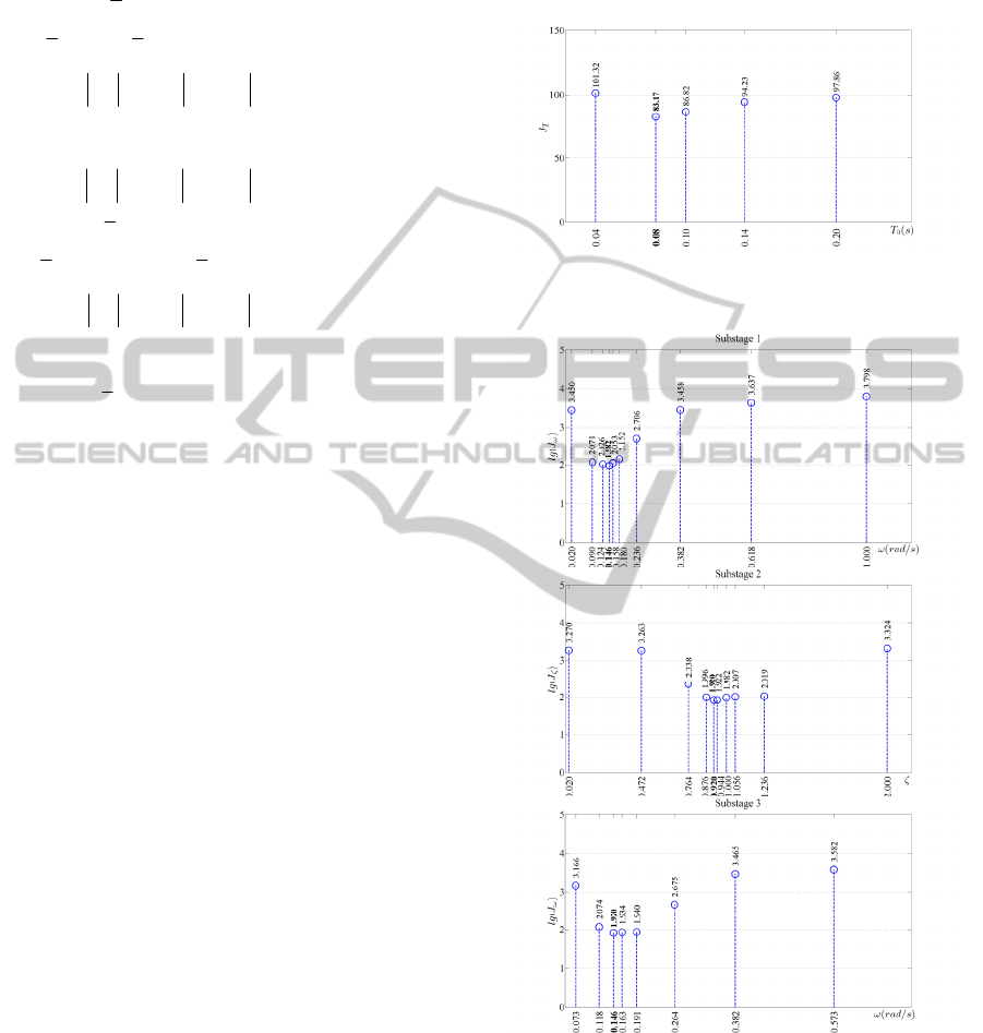
The searches of sampling period and closed-loop
parameters by golden section algorithm are depicted
in Figure 5 and Figure 6.
Figure 5: Search of sampling period (20) by golden
section algorithm.
Figure 6: Subcomponent search of closed-loop parameters
(28) by golden section algorithm with optimal sampling
period
s.08.0
*
0
T
Figure 5 demonstrates that the optimal sampling
period obtained by golden section algorithm is with
s.08.0
*
0
T
and Figure 6 depicts the search of closed-
loop parameters with that value of sampling period.
ICINCO2014-11thInternationalConferenceonInformaticsinControl,AutomationandRobotics
616
Notice that criterion, with a fixed sampling period to
its optimal value, is optimized within 3 steps of
subcomponent search procedure by golden section
algorithm thus is necessary to find only 28 criterion
values.
The optimization results by golden section
algorithm have shown that optimal closed-loop
parameters and optimal sampling period are
,rad/s146.0
*
,92.0
*
s.08.0
*
0
T
with minimal
criterion value
,17.83
*
Q
when
9
(
,90.81
*
Q
when
0
).
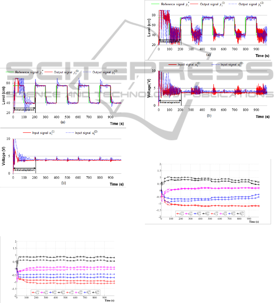
The control performance of digital self-tuning
PID control of pressure process with optimal closed-
loop parameters and optimal sampling period is
demonstrated in Figure 7. The on-line identification
of model parameters of this case is illustrated in
Figure 8.
Figure 7: Control performance of self-tuning PID control
of pressure process with optimal closed-loop parameters
and optimal sampling period -
,rad/s146.0
*
,92.0
*
s.08.0
*
0
T
, (a) – reference and output signals, (b) –
control signals.
Figure 8: On-line identification of model parameters –
self-tuning PID control with optimization.
If we select slightly shifted values from optimal
closed-loop parameters (
,rad/s174.0
)0.1
with
sampling period remaining unchanged, the control
performance by self-tuning PID control (Figure 9) is
degraded - the steady state error is significantly
increased and the variance of control signals change
are also raised. The on-line identification of model
parameters of this case is illustrated in Figure 10.
Figure 9: Control performance of self-tuning PID control
of pressure process with closed-loop parameters and
sampling period -
,rad/s174.0
,0.1
s.08.0
*
0
T
, (a)
– reference and output signals, (b) – control signals.
Figure 10: On-line identification of model parameters –
self-tuning PID control.
The sampling period (
0
T
) is commonly selected
from equation (Åström and Wittenmark, 1997)
,6.01.0
0
T
(46)
but optimization results show that with optimal
closed-loop parameters and sampling period is
outside of the interval (46). Figure 11 demonstrates
that with unoptimal sampling period, from the
interval (46), the control quality of pressure process
is significantly decreased.
DigitalSelf-tuningControlforPressureProcess
617
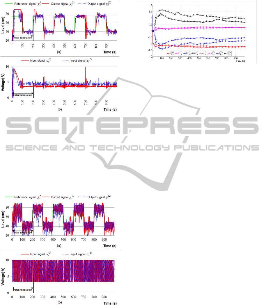
Figure 11: Control performance of self-tuning PID control
of pressure process with closed-loop parameters and
sampling period -
,rad/s118.0
,662.0
s.0.1
0
T
, (a)
– reference and output signals, (b) – control signals.
The control performance of pressure process by
predictor-based self-tuning controllers with
constraints is depicted in Figure 12. It is seen from
the graph that control quality is poor: the output
signals of both tubes not settle in certain time,
oscillating with high amplitudes.
Figure 12: Control performance of predictor-based self-
tuning control with constraints for pressure process with
s.,1.0
0
T
V,5.3
)(
min
i
u V,10
)(
max
i
u V10
)(
i
t
:
,9.2675Q
when
9
(
,02.186Q
when
0
), (a) – reference and
output signals, (b) – control signals.
The on-line identification of model parameters of
this case is illustrated in Figure 13.
Figure 13: On-line identification of model parameters –
predictor-based self-tuning control with constraints.
Considering only the variance of control errors, i.e.
not taking into account the influences of control
signals from criterion (19), the optimized self-tuning
PID control (Figure 7) has up to 2 times lower as
compared to predictor-based self-tuning control with
constraints (Figure 12).
6 CONCLUSIONS
The design method of digital self-tuning PID control
with optimization of closed-loop parameters and
sampling period for pressure process has been
proposed.
The multidimensional optimization problem of
closed-loop parameters and sampling period by
subcomponent search method may be divided into
optimization problems of one-variable functions.
The predictor-based self-tuning control with
constraints for both - minimum-phase and
nonminimum-phase - process models is proposed.
Experimental analysis has demonstrated that the
control quality of pressure process by digital self-
tuning PID control with closed-loop parameters and
sampling period optimization is significantly better
as compared to the predictor-based self-tuning
control with constraints.
REFERENCES
Åström, K., J., Hagglund, T., 1995. PID Controllers:
Theory, Design, and Tuning, Research Triangle Park,
North Carolina.
Åström, K., J., Hagglung, T., 2001. The future of PID
control. In Control Engineering Practice, vol. 9, no.
11, pp. 1163-1175. ScienceDirect.
Åström, K., J., Wittenmark, B., 1980. Self-tuning
controller based on pole-zero placement. In IEE
Proceedings D, vol. 127, pp. 120-130. IEEEXplore.
Åström, K., J., Wittenmark B., 1997. Computer-
Controllers Systems: Theory and Design, Prentice
ICINCO2014-11thInternationalConferenceonInformaticsinControl,AutomationandRobotics
618

Hall, New Jersey, 3
rd
edition.
Bobál, B., Böhm, J., Fessl, J., Macháček J., 2005. Digital
Self-tuning Controllers, Springer-Verlag. London, 2
nd
edition.
Boucher, A., R., Cox, C., S., Doonan, A., 1989. Sampling
Time Selection and its Effect on Direct Digital
Adaptive Control Algorithm Implementation. In IEE
Colloquium on Implementation Problems in Digital
Control, pp. 5/1-5/8. IEEEXplore.
Isermann, R., 1991. Digital Control Systems, Springer-
Verlag. London, 2
nd
edition.
Kaminskas, V., 1982. Dynamic system identification via
discrete-time observation: Part 1. Statistical method
foundation. estimation in linear systems, Mokslas
Publishers. Vilnius (in Russian).
Kaminskas, V., 2007. Predictor-Based Self Tuning
Control with Constraints. In Book Series Springer
Optimization and Its Applications, Model and
Algorithms for Global Optimization, vol. 4, p. 333-
341.
Kosorus, H., Hollrigl-Binder, M., Allmer, H., Kung, J.,
2012. On the Identification of Frequencies and
Damping Ratios for Structural Health Monitoring
Using Autoregressive Models. In 23rd International
Workshop on Database and Expert Systems
Applications (DEXA), pp. 23–27. IEEEXplore.
Levine, W., S., 1999. The Control Handbook. CRC Press,
Mumbai.
Levine, W., S., 2011. The Control Handbook, Second
Edition: Control System Fundamentals, CRC Press.
London, 2
nd
edition.
Liaucius. G., Kaminskas, V., Liutkevicius, R., 2011.
Digital Self-Tuning PID Control of Pressure Plant
with Closed-Loop Optimization. In Information
Technology and Control, vol. 40, no. 3, pp. 202 209.
Liaucius, G., Kaminskas, V., 2012. Adaptive digital PID
control of pressure process. In Power Engineering,
vol. 58, no. 3, pp. 158-165. EBSCO.
Liaucius, G., Kaminskas, V., 2012. Closed-Loop
Optimization Algorithms in Digital Self-Tuning PID
Control of Pressure Process. In ECT2012 – the 9th
International Conference on Electrical and Control
Technologies, pp. 25–29.
Ortega, R., Kelly, R., 1984. PID self-tuners. Some
theoretical and practical aspects. In IEEE Transaction
of Industrial Electronics, vol. 31, pp. 332-338.
IEEEXplore.
Vu, V., H., Thomas, M., Lakis, A., A., Marcouiller, L.,
2007. Multi-autoregressive model for structural output
only modal analysis. In Proceedings of the 25th
Seminar on machinery vibration, Canadian Machinery
Vibration Association, pp. 41-1.
DigitalSelf-tuningControlforPressureProcess
619
