
Optimizing Camera Placement in Motion Tracking Systems
D´avid Szal´oki, Krist´of Csorba, G´abor Tevesz
Department of Automation and Applied Informatics, Budapest University of Technology And Economics,
Magyar Tud´osok k¨or´utja 2/Q., H-1117 Budapest, Hungary
Keywords:
Localization Accuracy, Multi-Camera System, Motion Tracking, Optimal Camera Placement.
Abstract:
This paper discusses the placement of cameras in order to achieve the highest possible localization accuracy.
It is reached by using several cameras with redundant fields of views. A camera model is introduced and the
components which cause the localization errors are identified. The localization accuracy measure is defined
for one and for multiple cameras too. The problem of adding a new camera to the system in order to improve
the accuracy is formulated. The method for finding the optimal placement of this new camera is presented.
Some features are enumerated which can be applied for getting an advanced method.
1 INTRODUCTION
Object tracking is nowadays a very popular segment
of computer vision. There are application where mul-
tiple cameras are used to perform this task. The ap-
plications can be separated based on the common field
of views of the cameras. The first class contains ap-
plications with relatively few overlapping in the field
of views. This class contains applications like video
surveillance systems where the observed area can be
maximized. With these systems the object tracking
has to be performed with low accuracy requirements.
Only the approximated trajectory is interesting like
in (Zhou and Aggarwal, 2006), not its accuracy.
The second class contains applications where the
localization accuracy can be helpful. There are a lot
of algorithms for the PnP problem which stands for
Perspective-n-Point problem meaning the estimation
of the pose of a calibrated camera from n 3D-to-
2D point correspondences. There are several papers
about the solution of the P3P, P4P or the general-
ized PnP problem. Some of them originate the PnP
problem in the simpler ones. There are given for this
estimation iterative (Oberkampf et al., 1996) and non-
iterative (Hesch and Roumeliotis, 2011) (Moreno-
Noguer et al., 2007) methods as well. In applications
using feature point-based camera tracking (Skrypnyk
and Lowe, 2004) (Lepetit and Fua, 2006) dealing with
hundreds of noisy feature points is required. Detailed
summary about the PnP can be found in (Wu and Hu,
2006). All of these generalized methods can be im-
proved if the nature of the noise is known. Thus our
first goal is to determine the localization accuracy.
The calculated localization accuracy can be used to
validate the measured localization accuracy as pre-
sented in (Szal´oki et al., 2013a).
Another popular topic is the object tracking where
a high localization accuracy is required. There are ap-
plications where only the object locations are used.
If the variation of the localization could be supplied
the system performance could be improved. A typical
application is the robotic football contest (K¨appeler
et al., 2010). Here the ball is tracked with stereo cam-
eras. There are competitions where a prebuilt multi-
camera system can be used by the teams. With this
both the ball and the players can be recognized and
tracked. The information about the localization ac-
curacy could be useful for precision positioning and
aiming.
In (Ercan et al., 2007) a room is built with multiple
fixed cameras. An object is tracked while it can be
hidden by some other objects from several cameras.
In this case the experimental result could be validated
with the theory of localization accuracy.
Assume that we have a camera system containing
fixed and movable cameras. We would like to track
an object in the world as accurately as possible. The
movable cameras can be placed by the system opti-
mally so that the localization accuracy gets it’s high-
est possible value. The position and orientation con-
straints of the movable cameras are the limitations.
We would like to suggest a method for placing the
movable cameras in order to get the highest possible
localization accuracy.
288
Szalóki D., Csorba K. and Tevesz G..
Optimizing Camera Placement in Motion Tracking Systems.
DOI: 10.5220/0005012202880295
In Proceedings of the 11th International Conference on Informatics in Control, Automation and Robotics (ICINCO-2014), pages 288-295
ISBN: 978-989-758-040-6
Copyright
c
2014 SCITEPRESS (Science and Technology Publications, Lda.)
At first a camera model has to be formulated. The
components which cause the localization inaccuracy
can be identified. The localization accuracy has to be
defined and a measure has to be chosen. The nature
of these has to be examined for better understanding
their behavior. As a first step they can be formulated
in 2D for one observed point. Later this model can
be generalized into 3D and for an observed area or
volume instead of one observed point. Finally, some
extra features can be included as the field of view, the
dynamic constraints or the optimization of more than
one cameras together.
Please note that the presented algorithms and
methods are part of the Smart Mobile Eyes for Local-
ization (SMEyeL) system which is open-source and
is written in C++ using the popular OpenCV (Brad-
ski, 2000) computer vision library. The source code,
documentation and all the input data for the presented
measurements are available for download from our
homepage (SMEyeL, 2013).
2 LOCALIZATION ACCURACY
We assume that we use calibrated cameras. A cali-
brated camera represents a model, where the distor-
tions are identified and the pinhole camera model is
approximated during the mapping. Detailed informa-
tion about the camera model and the calibration pro-
cess can be found in (Bradski and Kaehler,2008). The
object localization has a finite accuracy, but then why
do we have localization error?
2.1 No Depth Information
One camera by itself can not provide depth informa-
tion. Based on the image of one camera only a half
line can be calculated on which the object is located.
Using every half line calculated from every camera
can be lead to localize the object. Of course in the
real world these half lines do not intersect in a sin-
gle point. Thus an optimal solution has to be found
which can be defined as the object location. Detailed
calculations and experimental results can be found
in (Szal´oki et al., 2013a).
2.2 Detection Error
One camera can detect the tracked object on its own
image with an error. This is defined as the detection
error. The further the object is, the larger the relative
error gets.
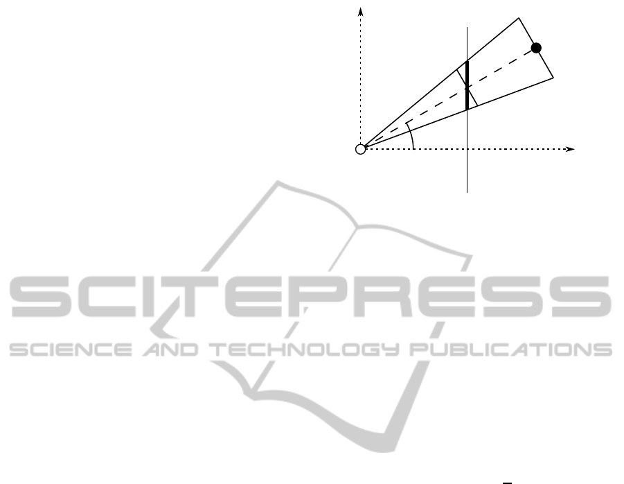
The derivation of the localization error in 2D can
be followed in Fig. 1. This figure is distorted for the
σ
⟂
φ
e
x
(c)
x
y
e
⟂
f
Figure 1: The derivation of the localization error from the
detection error. The camera is symbolized with the empty
circle. It is facing into the direction x and it has an imager
represented by a thin vertical line. f is the focal length. The
object is the filled circle which is located at the point x
x
x
(c)
in the camera coordinate system. The object is detected by
the camera at ϕ angle. The detection error e has a perpen-
dicular component e
⊥
. The perpendicular component of the
localization error is σ
⊥
.
sake of illustration, but in reality the focal length is
much larger than the detection error. This means that
the following assumption is a good approximation:
e
⊥
≈ e·cosϕ. (1)
This error is scaled up to the object location, so:
σ
⊥
≈ d · cos
2
ϕ·
e
f
, (2)
where f is the focal length and e is the detection er-
ror of the camera. The distance of the object from
the camera is d. ϕ is the detection angle and σ
⊥
is
the perpendicular component of the localization er-
ror. Assuming that the camera is facing towards the
tracked object this means that the perpendicular com-
ponent of the standard deviation is proportional to the
distance of the object.
2.3 Covariance Matrix
Therefore, we can calculate the perpendicular compo-
nent of the localization error of one camera at a single
point. As shown in section 2.1 one camera can not
provide depth information. This means that the paral-
lel component of the localization error is:
σ
k
→ ∞. (3)
For a point in the real world a matrix similar to
a covariance matrix can be formulated using (2) and
(3). This matrix is diagonal in the coordinate system
fitted to the facing direction of the camera and it can
OptimizingCameraPlacementinMotionTrackingSystems
289
be easily transformed (rotated) into the world coordi-
nate system:
Σ
Σ
Σ = R
R
R
T
α
R
R
R
ϕ
σ
2
k
0
0 σ
2
⊥
R
R
R
T
ϕ
R
R
R
α
, (4)
where α is the orientation of the camera and ϕ is the
detection angle. R
R
R
α
and R
R
R
ϕ
are the rotation matrices
in 2D with angle α and ϕ respectively. σ
k
and σ
⊥
are the parallel and perpendicular components of the
localization error.
2.4 Using Multiple Cameras
It has been previously shown that the covariance ma-
trix for one camera observing one single point can
be calculated. If more than one camera is used, for
each camera its covariance matrix can be determined.
These matrices can be combined into one matrix con-
taining the variances of the resulting localization er-
ror. This can be achieved by applying the following
formulas incrementally:
Σ
Σ
Σ
c
=
Σ
Σ
Σ
−1
1
+ Σ
Σ
Σ
−1
2
−1
, (5)
µ
µ
µ
c
= Σ
Σ
Σ
c
·
Σ
Σ
Σ
−1
1
µ
µ
µ
1
+ Σ
Σ
Σ
−1
2
µ
µ
µ
2
, (6)
where the two original densities are N (µ
µ
µ
1
, Σ
Σ
Σ
1
) and
N (µ
µ
µ
2
, Σ
Σ
Σ
2
), while the combined density is N (µ
µ
µ
c
, Σ
Σ
Σ
c
).
This is the so called product of gaussian densities.
0 50 100 150
−60
−40
−20
0
20
40
60
x
y
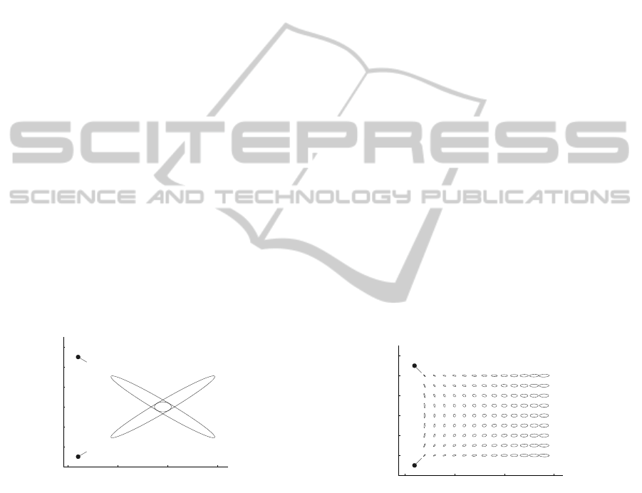
Figure 2: The derivation of the combined covariance ellipse.
Two cameras are observing one single point. The cameras
are represented with filled circles. The two larger ellipses
are the individual covariance ellipses of the cameras sepa-
rately. For better visualization their major axes are shrunk
so that not only two pairs of parallel lines can be seen. The
smaller ellipse is the combined covariance ellipse.
A simple example is shown in Fig. 2. The filled
circles are the cameras and the short line segments
symbolize their directions. The covariance ellipses
are drawn at a confidence level of 95 %. The two
larger ones are the original ellipses of the cameras.
They are distorted, since the limit of their major axis
is ∞, but in the figure these axes are chosen in such
a way that not only two pairs of parallel lines can be
seen. The smaller ellipse is the resulting covariance
ellipse. This is not distorted and it can be observed,
that the large localization error of one camera disap-
peared, as the resulting ellipse is smaller.
It can be noticed that the original covariance ma-
trix of one camera contains an element which ap-
proaches ∞. Despite this, the inverse of this matrix
can be calculated and contains only finite elements.
According to (5) the inverse of the final resulting co-
variance matrix is:
Σ
Σ
Σ
−1
r
=
n
∑
i=1
Σ
Σ
Σ
−1
i
, (7)
where n is the number of the cameras used for local-
ization and Σ
Σ
Σ
−1
i
is the inverse of the covariance matrix
of the i
th
camera. Since (7) contains only the inverse
matrices the inverse of the resulting matrix can be cal-
culated and it contains only finite elements. The de-
terminant of this matrix is zero if and only if there is
a specific direction in space in which the localization
has a variancewith unboundedlimit. This can occur if
the observed point and the centers of all the cameras
fit on the same line. If the determinant of this ma-
trix is non-zero, the resulting covariance matrix can
be calculated and the localization has a finite variance
in every direction.
In Fig. 3 a camera configuration and the resulting
covariance ellipses can be seen. The placement of the
ellipses is symmetric, since all the cameras have the
same parameters. It can be seen that the errors near
0 50 100 150
−60
−40
−20
0
20
40
60
x
y
Figure 3: The resulting covariance ellipses of the localiza-
tion using a specific camera configuration.
the cameras are smaller and they have a larger vari-
ance in the y direction, while the distant ones have the
larger variance in the x direction.
The next step is to define a way to measure how
good the localization is if the tracked object is located
in a single observed point. This measure is the lo-
calization accuracy and it can be defined in various
ways. In this paper two methods are discussed. In
both cases the accuracy is derived from the inverse of
resulting covariance matrix. The inverse is used be-
cause in some cases the inverse exists but the original
matrix does not.
ICINCO2014-11thInternationalConferenceonInformaticsinControl,AutomationandRobotics
290
2.4.1 Determinant as Measure of Quality
First we can define the accuracy as the determinant of
the inverse covariance matrix:
q
det
=
Σ
Σ
Σ
−1
r
, (8)
where q
det
stands for quality using the determinant.
This measure has a physical meaning as it is inversely
proportional to the area of the covariance ellipse.
0
50
100
150
−50
0
50
0
0.5
1
1.5
2
2.5
3
x 10
4
x
y
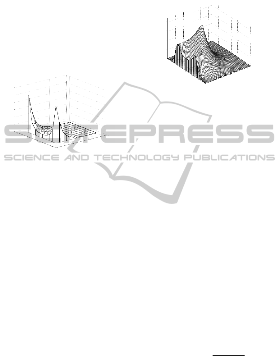
Figure 4: The surface plot of the accuracy in 2D using the
previous camera configuration (the same as in Fig. 3) and
the determinant measure. The measure is defined in (8).
In Fig. 4 the accuracy is presented in the case of
the previous camera configuration. It can be noticed
that the closer the observed point is, the better the ac-
curacy becomes. This occurs because the accuracy is
proportional to the inverse of the distance (d
−1
). Of
course an object can not be placed arbitrarily close to
one of the cameras because a camera has a physical
size and minimal focal distance.
2.4.2 Eigenvalue as Measure of Quality
Another possibility is to define the quality as the worst
case:
q
eig
= min
eig
Σ
Σ
Σ
−1
r
, (9)
where Σ
Σ
Σ
−1
r
is the inverse of the resulting covariance
matrix. q
eig
is the smallest eigenvalue of the inverse
matrix. This measure also has a physical meaning as
it is proportional to the largest axis of the ellipse.
In Fig. 5 the accuracy is presented in the case of
the previous camera configuration using the smallest
eigenvalue of the inverse covariance matrix as mea-
sure. This is different from Fig. 4, where the deter-
minant was used as measure. Here the best quality is
achieved at a point where the detection directions of
the two cameras are perpendicular.
20
40
60
80
100
−60
−40
−20
0
20
40
60
20
40
60
80
x
y
Figure 5: The surface plot of the accuracy in 2D using the
previous camera configuration (the same as in Fig. 3) and
the eigenvalue measure. The measure is defined in (9).
3 ADD ONE CAMERA
Let there be given a set of fixed cameras to define the
camera configuration. These cameras are used for lo-
calization at a given point. We would like to add a
new camera to the system. The general problem is:
how should we place the new camera in order to in-
crease the accuracy as much as possible.
The common method is:
1. Calculate the covariance matrix of the localization
determined by the fixed cameras at the observed
point.
2. Calculate the covariance matrix parametrized for
the new camera at the observed point.
3. Combine these two matrices using (5).
4. Calculate the objective function (q) defined in (8)
or in (9).
5. Find the extremal points of this objective function.
Assume that the new camera is placed so that it is
facing into the direction of the observed point.
3.1 Using the Determinant Based
Measure
In this case the previously described method is used
with the determinant measure defined in (8). The lo-
calization accuracy in the polar coordinate system fit-
ted to the covariance ellipse generated by the fixed
cameras is:
q
det
(α, d) = C+
B+ A· sin
2
α
d
2
, (10)
where α and d are the angle and distance in the po-
lar coordinate system. A, B and C are constant non-
negative values which are functions of the camera pa-
rameters and the fixed cameras (Szal´oki et al., 2013b).
OptimizingCameraPlacementinMotionTrackingSystems
291
This means that if the new camera is placed at the
(α, d) point the localization accuracy at the origin is
equal to q
det
.
This formula can be easily converted into the
cartesian coordinate system:
q
det
(x, y) =
A· y
2
(x
2
+ y
2
)
2
+
B
x
2
+ y
2
+C, (11)
where x and y are the coordinates of the new camera.
A, B and C are the previously mentioned constant val-
ues.
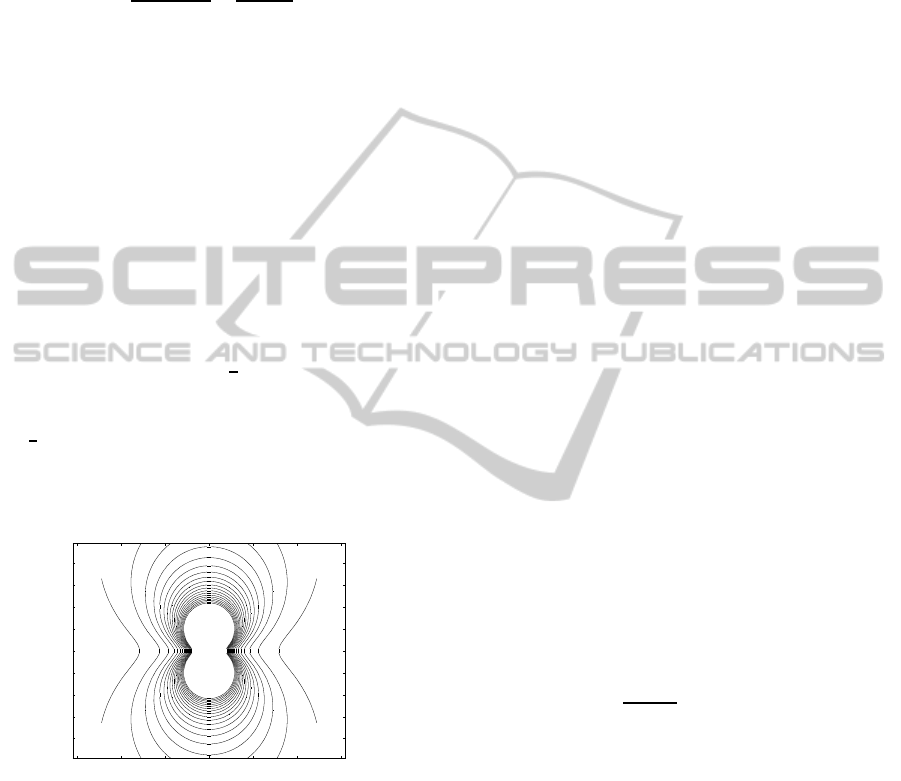
In Fig. 6 the contour of a specific case is plotted.
The same two cameras as in Fig. 3 observe the ori-
gin and a new camera is added. The curves are “iso-
accuracy” curves which means that if the new cam-
era is placed anywhere on a curve the resulting local-
ization accuracy becomes the same value. A curve
contained by another one has a higher localization ac-
curacy. It can be noticed from (11) that the plot has
reflectional symmetry with the x and y axes as well.
In this case the covariance matrix generated from the
fixed cameras has two eigenvalues which rate is 1 to
3. If this rate is smaller than
1
2
, the contour plot be-
comes similar: q
det
has two local maxima, accord-
ing to the partial derivative by y. If the rate is larger
than
1
2
, the curves become convex ones and q
det
has
only one local maximum using a fixed y. Detailed
calculations and experimental results can be found
in (Szal´oki et al., 2013b).
x
y
−60 −40 −20 0 20 40 60
−40
−30
−20
−10
0
10
20
30
40
Figure 6: The contours of the localization accuracy with the
newly added camera. The covariance matrix of the local-
ization generated by some fixed cameras is known at the
origin. A new camera is added to the system. The value of
the localization accuracy with the new camera can be calcu-
lated. It is a function of the position of the new camera and
it has the same value along one curve. The closer the new
camera to the origin is, the higher the accuracy becomes.
3.2 Searching on the Boundary
Both of the partial derivatives of (11) equals zero only
at the origin, but a camera can not placed right at the
observed point. So this means that if a new camera is
placed with some constraints, the optimal placement
fits on the constraint boundary. This simplifies the
problem, since the extremal points of q
det
have to be
searched only on the boundary.
Another consideration can be that in the polar co-
ordinate system for any fixed α
0
:
q
det
(α
0
, d
1
) ≥ q
det
(α
0
, d
2
) ⇐⇒ d
1
≤ d
2
.
(12)
This results in the optimal placement fitting on the
constraint boundary since for any (α
0
, d
2
) point inside
the placing area there exists at least one point (α
0
, d
1
)
on the boundary where (12) is satisfied.
Assume that the boundary can be written as a
union of functions with one parameter:
[
i
{(x, y)|x = f
i
(t), y = g
i
(t), t ∈ [0..1]} (13)
If the extremal points are searched for on the i
th
boundary segment, the following has to be solved:
t
(opt)
= arg max
0≤t≤1
Q
i
(t), (14)
where
Q
i
(t) = q
i
( f
i
(t), g
i
(t)) = q
i
(x, y), (15)
which is the localization accuracy on the boundary
segment.
Unfortunately, on a boundary segment there can
be more than one local maximum even if the segment
is a simple line segment. So, global optimizers should
be started for every boundary segments. After that
the highest local maximum value can be chosen as a
global maximum.
Another possibility is to calculate the derivative
of Q
i
(t) on every boundary segment and find every t
value where:
∂Q
i
(t)
∂t
= 0. (16)
This can be a complex task, but fortunately, if the
boundary segments are line segments, this is reduced
to simple solving of third-degree polynomials, which
can be performed analytically. In this case the plac-
ing area of the new camera is a polygon. This polygon
limitation is not too strong since most of the bound-
aries can be approximated with polygons.
3.3 Using the Eigenvalue Based
Measure
Another possibility is to define the localization accu-
racy as q
eig
in (9). The characteristic polynomial of
the inverse covariance matrix can be formulated. The
smaller root of this polynomial is the accuracy. This
has to be maximized. In this case, if a new camera is
ICINCO2014-11thInternationalConferenceonInformaticsinControl,AutomationandRobotics
292

added in the polar coordinate system, the localization
accuracy is:
q
eig
(α, d) =
1
2
·
D+
F
d
2
−
r
F
2
d
4
+ E
2
+
2EF
d
2
· cos(2α)
!
,
(17)
where D, E and F are constant non-negative values
which are functions of the camera parameters and the
fixed cameras. This equation can also be easily trans-
formed into the cartesian coordinate system, but it
gets a little long and it is not so interesting. One might
assume that if d → 0 then q
eig
→ ∞, but it is not true.
If d → 0 the members in the square root with d in
the denominator get dominant and they eliminate the
member with d in the denominator outside the root.
With substitution of the constant values, the inverse
of the originally smaller variance (most accurate di-
rection) gets the upper limit. This can be achieved if
the facing direction of the new camera is perpendicu-
lar to the direction of the most inaccurate direction.
x
y
−50 0 50
−50
−40
−30
−20
−10
0
10
20
30
40
50
Figure 7: The contours of the localization accuracy with
the newly added camera. A curve contained by another one
has a higher localization accuracy. The camera configura-
tion and camera parameters are the same as in Fig. 6. The
difference is that here the measure defined in (9) is used
instead of (8).
So the main difference from the previously dis-
cussed q
det
is that q
eig
has an upper limit while q
det
does not. While q
det
→ ∞ if d → 0, q
eig
has an up-
per limit. In Fig. 7 the contours of this function can
be seen. The camera parameters are the same as in
Fig. 6. The basic concept here is also correct that the
closer the camera is, the better the localization accu-
racy gets. However in this case it is more noticable
how powerful the angle is. If the new camera is placed
parallel to the most inaccurate direction, it improves
nothing, while with the determinant measure it does.
This behavior represents the real world better than the
determinant one.
In this case the optimal placement can also be de-
termined. A consideration similar to (12) can be for-
mulated here as well. This proves that if this line
segment and the placing area has no common point
it results that the optimum is situating on the bound-
ary. Unfortunately, the boundary can not be handled
so simply as in the determinant case because of the
square root in (17). This can be handled with global
optimization on the line segments. Although it is
resource-intensive, it is a simplified method since the
optimization has to be performed only on the line seg-
ments (1D) instead of the whole area (2D).
3.4 3 Dimensional Case
The previous sections focused on the 2D case. They
can be generalized to 3D by increasing the parame-
ter space. The result is that all the positions have
three coordinates instead of two. The orientation of
the camera is given with three angles rather than one,
thus the rotation matrices are the combination of three
rotations. There are two independent detection errors
and so two independent perpendicular components of
the localization accuracy. Thus the covariance matrix
is a 3-by-3 matrix instead of a 2-by-2 one. In 3D the
objective functions get more complex, specially the
measure with the eigenvalue. The optimization can
be done only numerically. A consideration similar to
(12) can be formulated here as well. This results in
the optimum lying on the boundary since the closer
point with the same orientation has a larger objective
funtcion value. Thus the optimization has to be per-
formed only on the 2D boundary instead of the whole
3D volume.
−40 −30 −20 −10 0 10 20 30 40
−30
−20
−10
0
10
20
30
Figure 8: The contours of the objective function defined
with the eigenvalue in 3D on a general plane. It has two
peaks and a hollow space between them. It means that the
angle is powerful and it can radically change the objective
function value on a short distance.
In Fig. 8 the contours of the objective function de-
fined with the eigenvalues can be seen on a general
plane. It has two peaks and a hollow space between
them. It means that there is a direction in which no
significant improvement can be achieved but with a
little shift in the angle the objective function increases
strongly.
OptimizingCameraPlacementinMotionTrackingSystems
293
4 EXPERIMENTAL RESULTS
We have developed a measurement to confirm the
localization accuracy theory presented in Section 2.
Three fixed, calibrated cameras observe a marker ob-
ject. The marker is represented by a printed im-
age that contains easily recognizable ellipses. This
marker is moved with a precision robotic arm into
each vertex of a 3-by-3-by-3cubic grid. Tens of local-
izations are performed at every position on the grid.
The mean of these measurements are used as estima-
tions of the positions. The localization accuracy can
be characterized by the standard deviation of these es-
timated marker locations. Detailed calculations, ex-
perimental setup and results can be found in (Szal´oki
et al., 2013a). The standard deviation of marker loca-
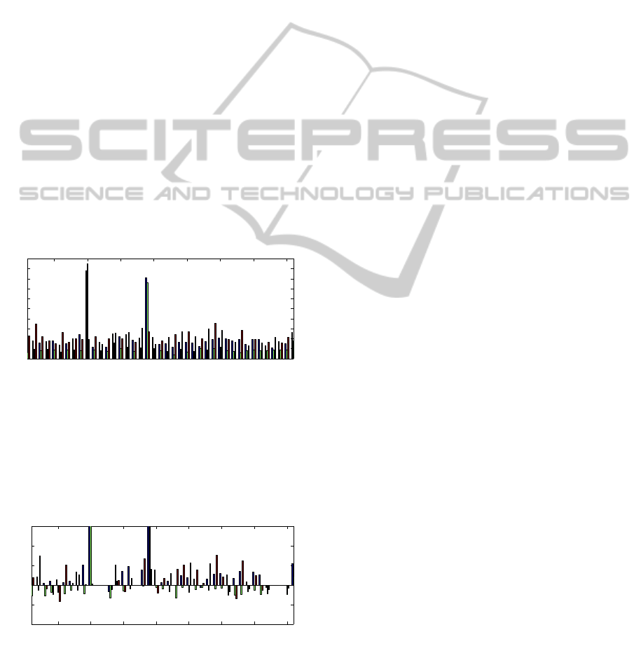
tion estimations can be seen in Fig. 9.
Fig. 10 shows the differences between the stan-
dard deviations of the theory and the measurement.
Based on our observations, the reprojection error sup-
plied by the OpenCV calibration method is a good
choice for estimating the detection error. The mea-
surement differs only with half of a millimeter from
the theory in most cases.
5 10 15 20 25 30 35 40
0
0.5
1
1.5
2
2.5
3
3.5
4
4.5
5
Location index
Standard deviation
Standard deviation (measurement)
Figure 9: Standard deviation of marker location estima-
tions, shown for the 3 axes separately. Differences are
caused by the varying view angles. The two large peaks
are measurement errors, they have to be ignored. The direc-
tion of the z axis is the nearest to the depth direction. This
confirms that the largest inaccuracy can be found in this di-
rection.
5 10 15 20 25 30 35 40
−1
−0.5
0
0.5
1
1.5
Location index
Standard deviation
Standard deviation (measurement−theory)
Figure 10: The standard deviation differences of the mea-
surement and the theory in each locations for the 3 axes
separately. The two large peaks are measurement errors, as
it is mentioned in Fig. 9.
5 FUTURE PLANS
In this section some features are listed which could
be applied to the model. Some of them are easy to
include but some cases need large changings and de-
velopments.
5.1 Area Instead of a Single Point
In the previous sections there is only one observed
point where the localization has to be performed. The
more general case is that the localization is needed
in an area. Therefore a density function can be used.
Its value at a specific x
x
x point in space represents the
probability that the localization has to be done at that
point. In this case the objective function can be de-
fined as the expected value of the accuracy:
E
x
x
x
(q(x
x
x)) =
Z
Ω
q(x
x
x) f (x
x
x) dx
x
x, (18)
where Ω represents the whole space and f (x
x
x) is the
density function.
Another method for handling not only one ob-
served point is, when the worst case is used. This
means that the localization accuracy on an area is de-
fined as the worst accuracy of its points.
5.2 Taking Field of View into Account
The field of view of the cameras can also be taken into
account. This is only a 0-1 function which multiplies
its inverse covariance matrix, but it complicates the
optimization. An idea is that the space can be cut into
pieces with the boundaries of the fields of views. One
piece can be handled as described previously and all
the pieces has to be managed individually.
5.3 Utilizing Multiple Cameras
Together
If multiple cameras can be placed for localization ac-
curacy improvementthen applying the previous meth-
ods means that the cameras are placed incrementally.
The resulting localization accuracy can be increased
by optimizing the movable cameras together.
5.4 Rotation in 3D
In 3D if the camera is placed at a fixed position so
that it is facing towards the observed point, then the
rotation around the facing direction can change the
objective function value. This rotation can also have
some constraints which have to be taken into account.
ICINCO2014-11thInternationalConferenceonInformaticsinControl,AutomationandRobotics
294

5.5 Continuous Optimization for
Dynamic Environments
Since a moving object is tracked the optimal place-
ment of the movable cameras should be performed
continuously through time. One camera can be placed
closer to the object in order to have larger accuracy
improvement, but if the object is moving fast it can
occur that the camera can not follow it because of
its dynamic constraints. It can be a better solution
to place the camera further in order to be able to fol-
low the object on a longer path. These dynamic con-
straints of the movable cameras could be also taken
into account.
6 CONCLUSIONS
In this paper the multi-camera localization accuracy
and the optimal camera placement is examined. First
the camera model is formulated. The localization ac-
curacy is defined for one camera observing one single
point. A method for calculating the localization ac-
curacy using multiple cameras is given. All the cal-
culations are performed in 2D and they are extended
later into 3D. Two measures are defined. Their ben-
efits and disadvantages are compared. In both cases
the objective function is calculated in case of adding
a new camera to the system. The optimization of the
placement of the new camera is discussed. The gen-
eral extension into 3D is described. Finally, the future
plans are formulated.
ACKNOWLEDGEMENTS
This work was partially supported by the Euro-
pean Union and the European Social Fund through
project FuturICT.hu (grant no.: TAMOP-4.2.2.C-
11/1/KONV-2012-0013) organized by VIKING Zrt.
Balatonf¨ured.
This work was partially supported by the Hungar-
ian Government, managed by the National Develop-
ment Agency, and financed by the Research and Tech-
nology Innovation Fund (grant no.: KMR 12-1-2012-
0441).
REFERENCES
Bradski, G. (2000). The OpenCV Library. Dr. Dobb’s Jour-
nal of Software Tools.
Bradski, G. and Kaehler, A. (2008). Learning OpenCV.
O’Reilly Media Inc.
Ercan, A., El Gamal, A., and Guibas, L. (2007). Object
tracking in the presence of occlusions via a camera
network. In Information Processing in Sensor Net-
works, 2007. IPSN 2007. 6th International Sympo-
sium on, pages 509–518.
Hesch, J. and Roumeliotis, S. (2011). A direct least-squares
(dls) method for pnp. In Computer Vision (ICCV),
2011 IEEE International Conference on, pages 383–
390.
K¨appeler, U.-P., H¨oferlin, M., and Levi, P. (2010). 3d object
localization via stereo vision using an omnidirectional
and a perspective camera.
Lepetit, V. and Fua, P. (2006). Keypoint recognition using
randomized trees. IEEE Trans. Pattern Anal. Mach.
Intell., 28(9):1465–1479.
Moreno-Noguer, F., Lepetit, V., and Fua, P. (2007). Accu-
rate non-iterative o(n) solution to the pnp problem. In
Computer Vision, 2007. ICCV 2007. IEEE 11th Inter-
national Conference on, pages 1–8.
Oberkampf, D., DeMenthon, D. F., and Davis, L. S.
(1996). Iterative pose estimation using coplanar fea-
ture points. Comput. Vis. Image Underst., 63(3):495–
511.
Skrypnyk, I. and Lowe, D. G. (2004). Scene modelling,
recognition and tracking with invariant image fea-
tures. In Proceedings of the 3rd IEEE/ACM Interna-
tional Symposium on Mixed and Augmented Reality,
ISMAR ’04, pages 110–119, Washington, DC, USA.
IEEE Computer Society.
SMEyeL (2013). Smart Mobile Eyes for Localization
(SMEyeL).
Szal´oki, D., Kosz´o, N., Csorba, K., and Tevesz, G. (2013a).
Marker localization with a multi-camera system. In
2013 IEEE International Conference on System Sci-
ence and Engineering (ICSSE), pages 135–139.
Szal´oki, D., Kosz´o, N., Csorba, K., and Tevesz, G. (2013b).
Optimizing camera placement for localization accu-
racy. In 14th IEEE International Symposium on
Computational Intelligence and Informatics (CINTI),
pages 207–212.
Wu, Y. and Hu, Z. (2006). Pnp problem revisited. J. Math.
Imaging Vis., 24(1):131–141.
Zhou, Q. and Aggarwal, J. (2006). Object tracking in
an outdoor environment using fusion of features and
cameras. Image and Vision Computing, 24(11):1244
– 1255. Performance Evaluation of Tracking and
Surveillance.
OptimizingCameraPlacementinMotionTrackingSystems
295
